Choosing the right Parameters

When you are starting out using the One AI extension you might wonder how to correctly set the parameters for your application. To help you get started, we collected several examples to give you a better idea on which setting works best for which tasks.

Overview of the Examples

Classification

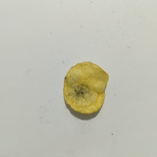
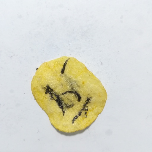
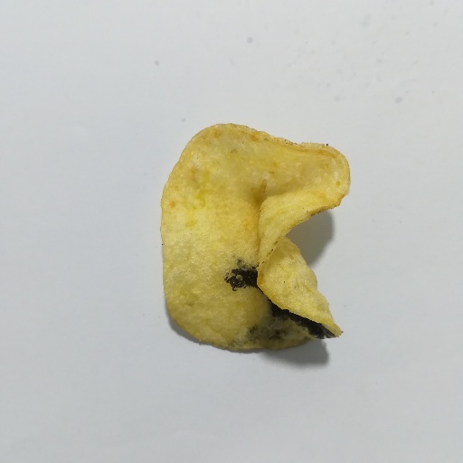
Potato Chips
This is the dataset we used in our Potato Chip Classification Demo. It contains images of good and burned potato chips that need to be classified for doing quality control. The burn marks can have different sizes and it's possible that the same chip has multiple burn marks.

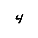
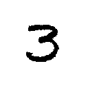
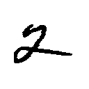
Handwritten Digits
The NIST Special Database 19, which we used in our Handwritten Digit Classification Demo, contains images of handwritten numbers. The goal of this demo is to classify the number that is visible in the image.

Screw Detection
The authors Yildiz and Wörgötter presented an approach for detecting screws in their paper DCNN-Based Screw Detection for Automated Disassembly Processes. They used a Hough Transform to detect circles and fed those images into a neural network to decide whether the candidate is a screw or an artifact. They provided a dataset that contains the detected candidates as well as labels whether the candidate is a screw or an artifact.

Object Detection

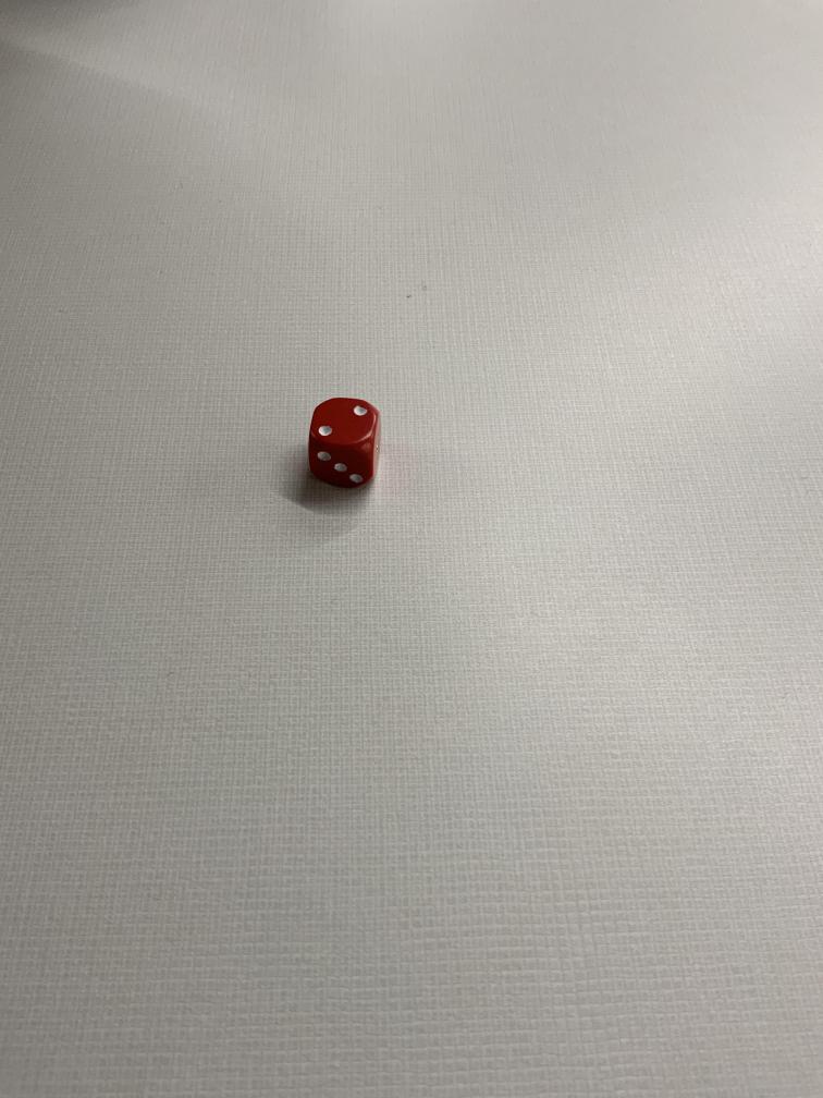
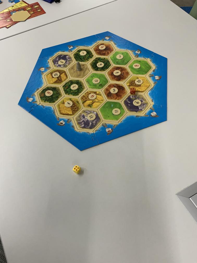
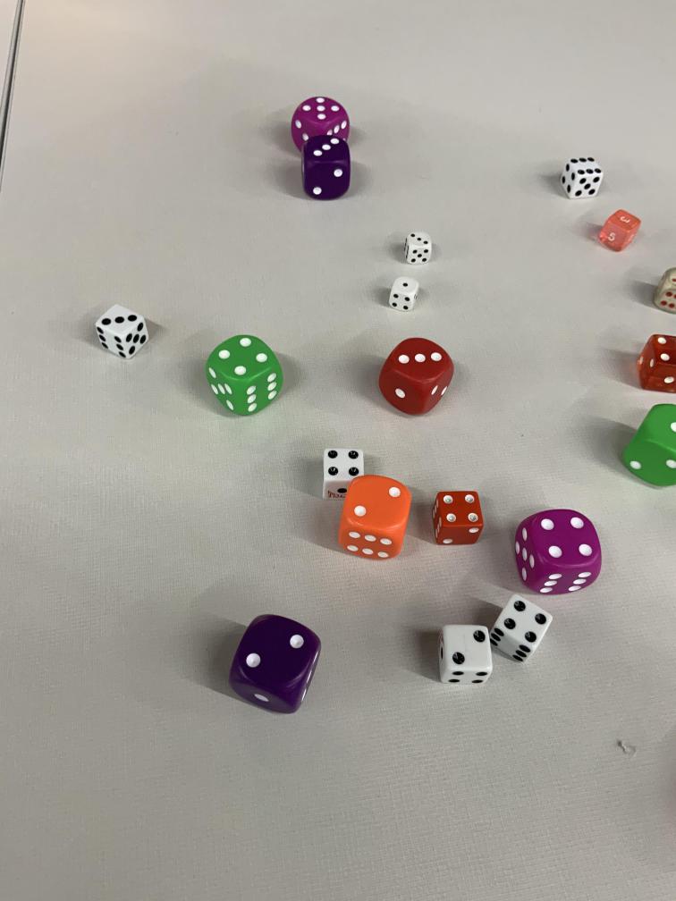
Dice
This is the dataset that was used in our Dice Detection Demo. It contains images of 6-sided dice that were positioned either on a white table or on a CATAN game board. The goal is to detect the position of the dice and predict the number that they are showing. There are also images containing a collection of varying dice.

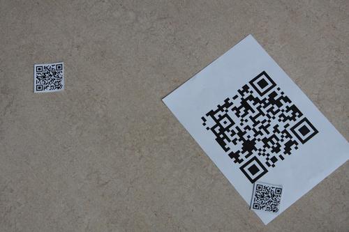
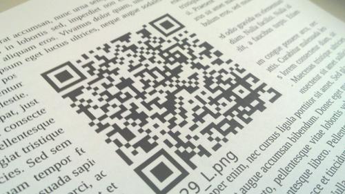
QR Code Detection
The images in this dataset contain one or multiple QR codes. The goal of this task is to predict the position and size of the different QR codes. Since the QR codes are passed into a separate application for processing afterwards, the precision of the predicted size and position aren't of great importance as long as the QR codes are detected.

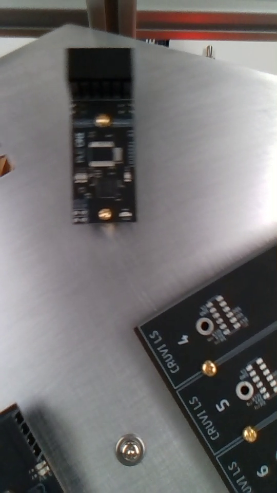
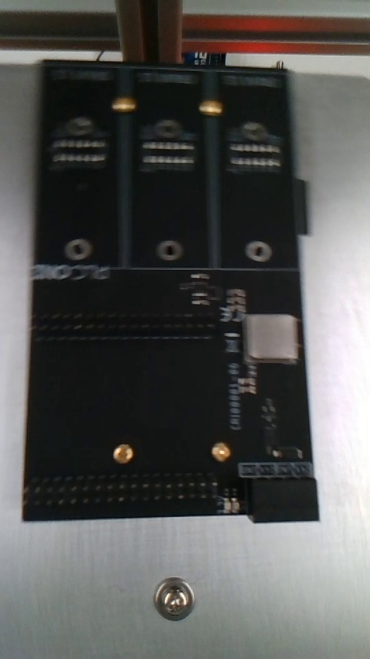
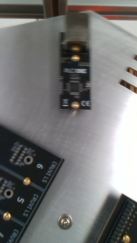
Detecting Components on Circuit Boards
This dataset contains images of circuit boards. The goal of this demo is to detect individual board components on the PCB in order to check whether all components are visible. Since the circuit boards were mounted on a spinning tray during the recording process, some parts of other PCBs might be visible in the images.

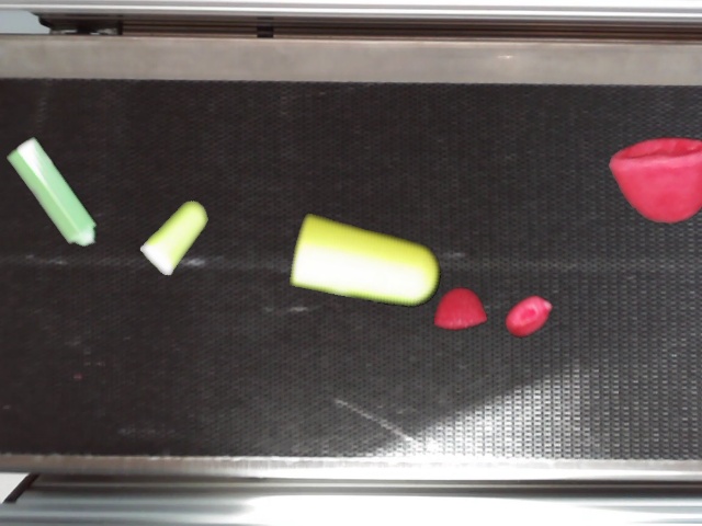
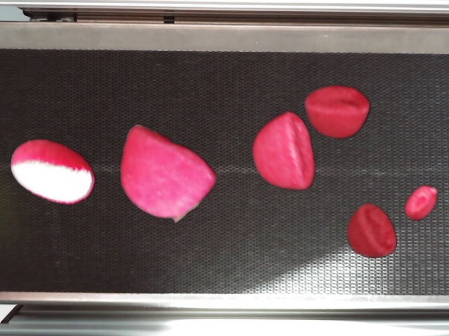
Conveyor Belt Detection
This dataset contains images that picture a conveyor belt transporting different kinds of demonstration objects. The goal of this demonstration is to detect the objects and differentiate between the strawberries and the foreign objects. A similar application might be used in the quality control process of a food processing production line.

Defect Detection on shiny Surfaces
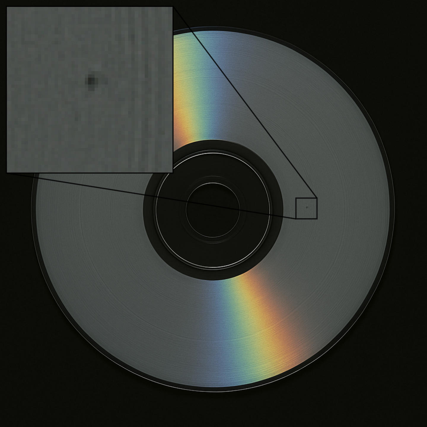
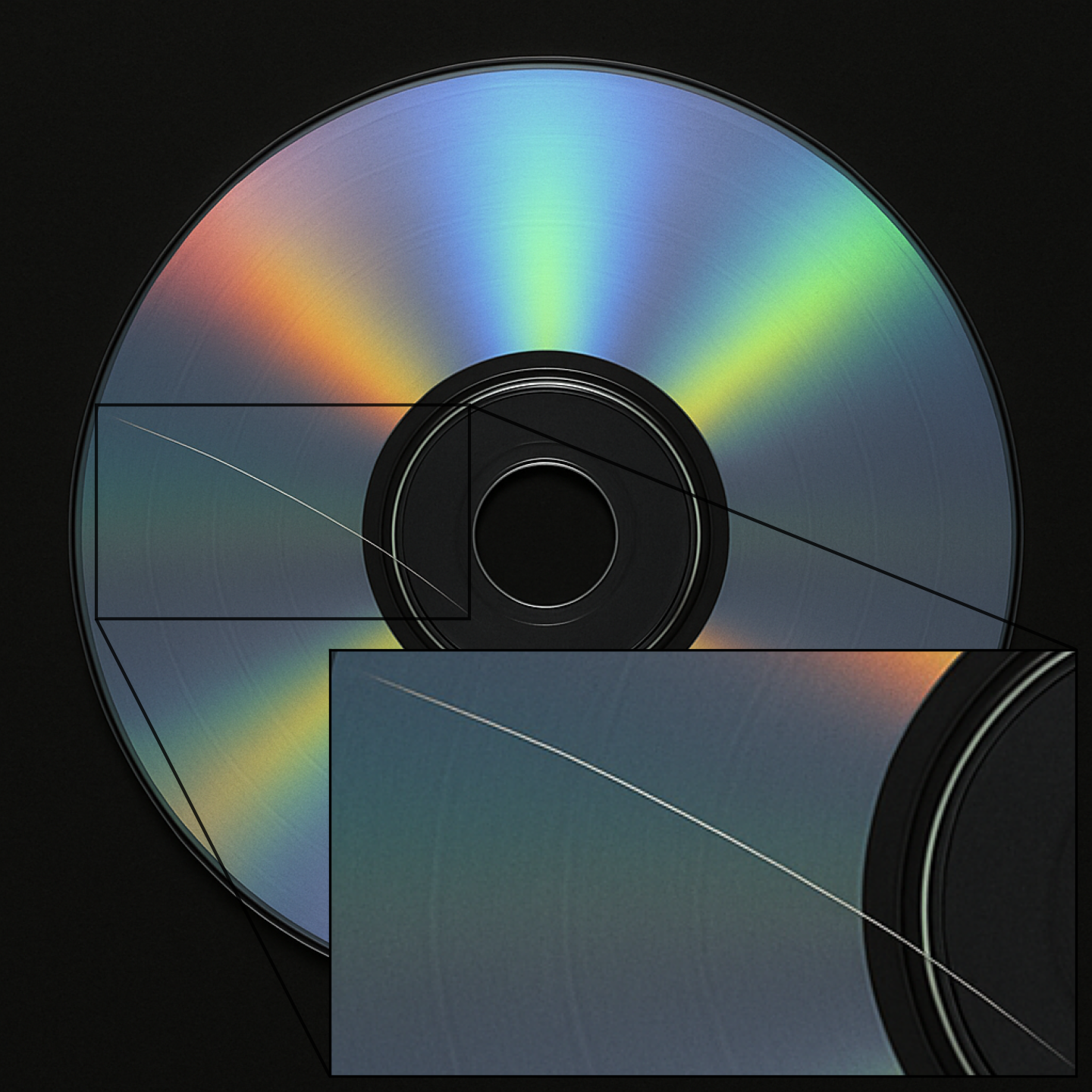
These images don't belong to an actual dataset but are a representation for the broader task of detecting defects on shiny metal surfaces. As you can see in the examples, the defects can range from tiny specs to huge scratches.

Model Settings

Output Settings

X/Y Precision (only used in Object Detection tasks)
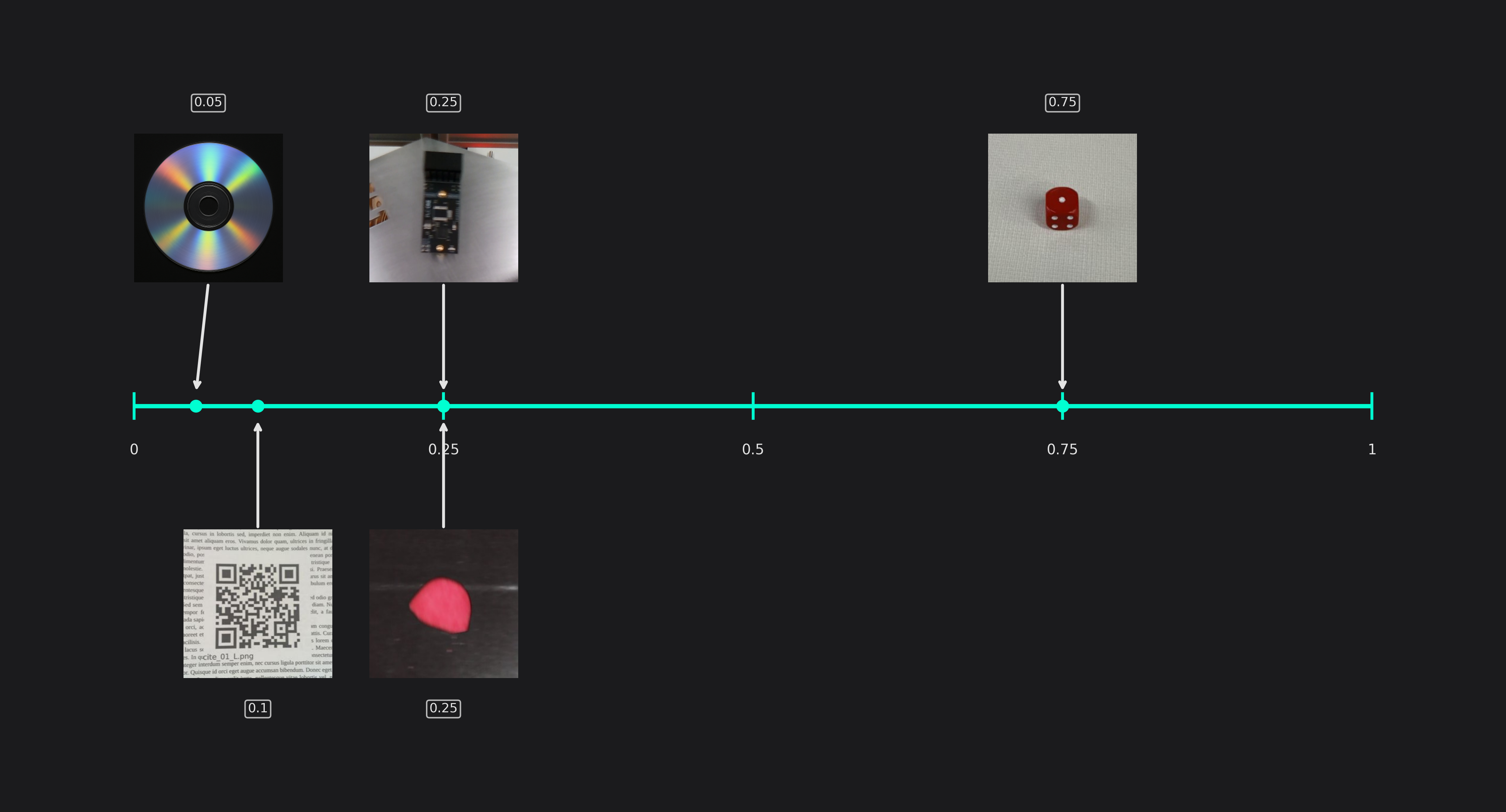
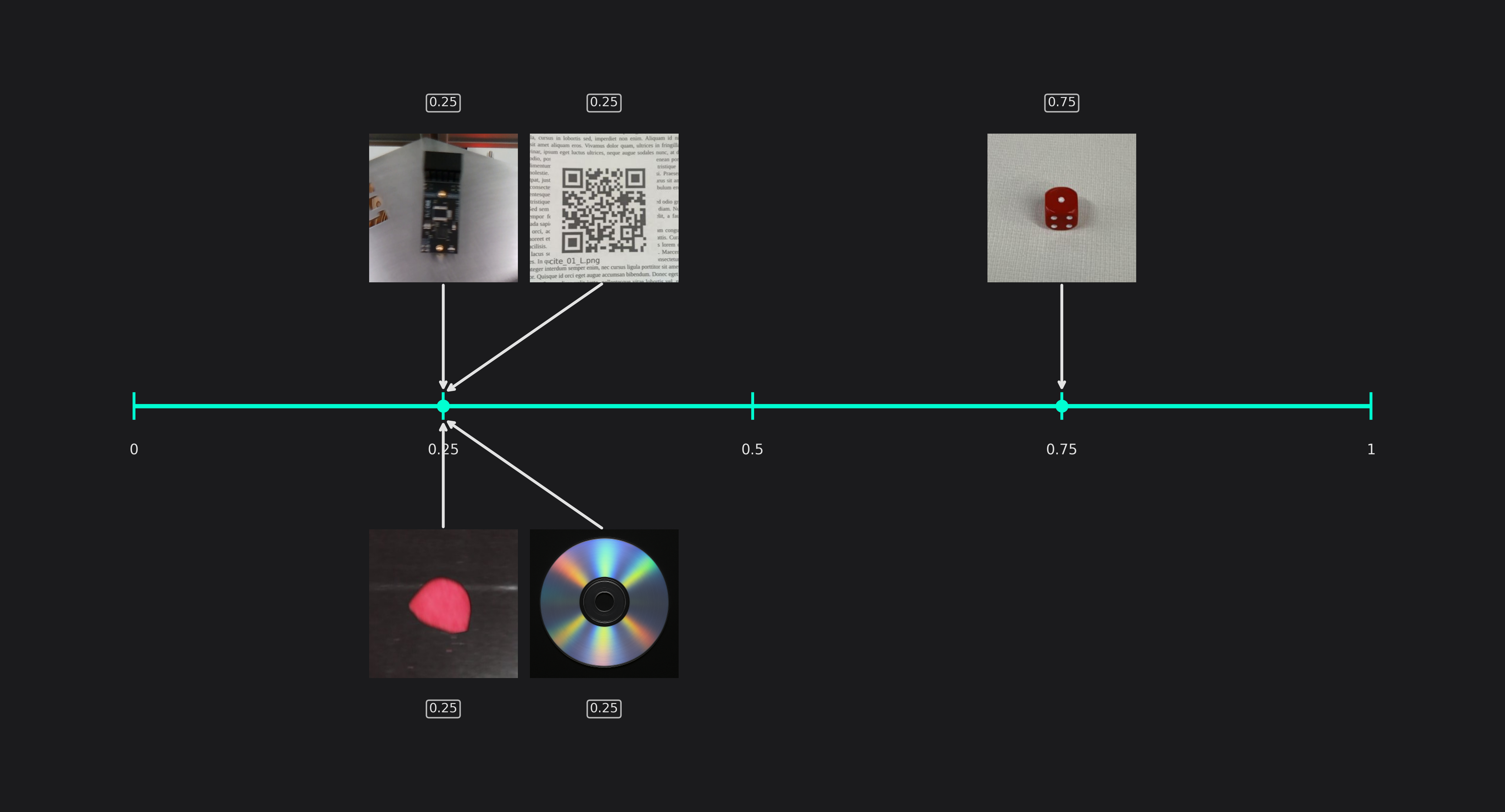
This setting allows you to control the precision of the predicted object locations. By reducing the X/Y precision, you effectively reduce its resolution. For example, if you set the X/Y precision to 25%, only every fourth pixel can be chosen as the position of a detected object. Objects that fall in between are still detected but the predicted positions won't be exact.
The advantage of reducing the X/Y precision is an increase in speed and for some applications even an improved generalization. This is especially useful for applications that don't require a highly precise position. For example, if we want to detect defects on metal surfaces, we are mainly interested in whether defects are present or not, but we don't need their pixel accurate position. The QR code example behaves similarly - since the detected QR codes are evaluated in a secondary step, their position doesn't need to be exact.

Size Precision (only used in Object Detection tasks)
You are also able to adapt the precision of the predicted object size to your needs. This setting directly controls the amount of computations that are spent on predicting the objects size, so a higher precision improves the predictions but increases the computational load.

Maximum Memory and Multiplier Usage
The settings for the maximum amount of memory and multipliers that are used by the AI don't rely solely on the task you want to solve but primarily on your hardware constraints. If you allow ONE AI to use more resources, it might be able to find a better model, but if you already have the best model for your constraints, additional resources won't be used.

Input Settings

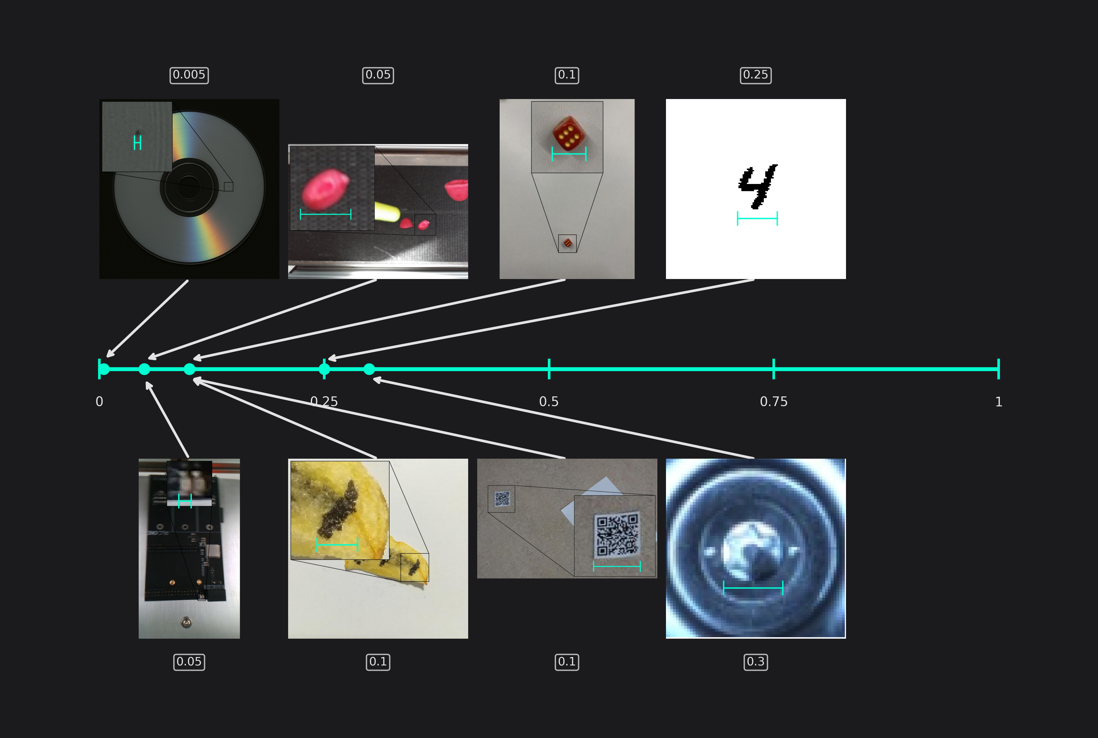
Estimated Surrounding Min Width and Height
These two settings describe the size of the area that the model needs to analyze to detect the smallest objects in your dataset correctly. For classification problems, it reflects the smallest relevant area that the model needs to analyze to make the correct decision. For most tasks, this area is equal to the size of the objects, but some tasks require the model to also analyze the area surrounding the object. For example, if you want to detect components on a PCB and decide whether they are installed incorrectly, you might need to also see its connecting traces and not just the component itself. Another example is the chips demo, where we set the estimated surrounding min width higher than the estimated min object width to prevent confusing shadows with burn marks.
When you enter different values for the width and height, please keep in mind that your objects might appear in a rotated orientation. For this reason, the estimated surround width and height are equal for many tasks even if the height and width of the actual objects aren't. If the objects in your task always appear in a similar orientation, you can tune these settings more precisely, resulting in unequal settings for width and height.
Another situation where the width and height are different occurs when your images aren't square. For example, if your image is twice as wide as it's high, your estimated width will be half of the estimated height for square objects. Because of the unequal image dimensions, the differing relative lengths correspond to equal lengths when measured in pixels.
You don't need to worry about combing through your whole dataset to find the smallest and the largest samples. Giving a reasonable estimate is sufficient for achieving good results.
For the sake of brevity, the following examples will only show the setting for the object width.

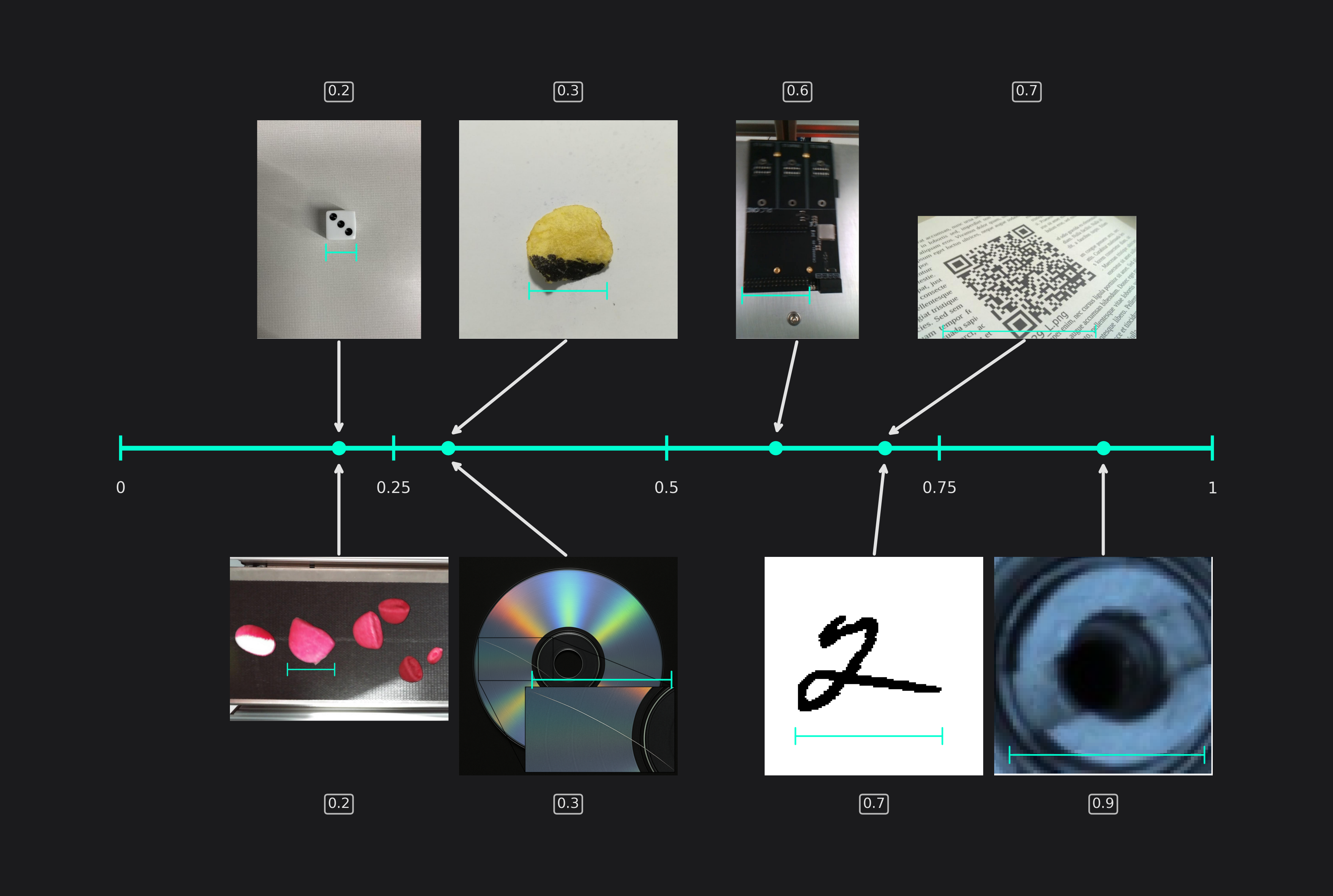
Estimated Surrounding Max Width and Height
Equivalent to the previous setting, this setting specifies the size of the area that the model needs to analyze to detect the largest objects. For classification tasks, it specifies the largest relevant area for making a decision instead.
(Please note that some of the images in the other example have been cropped for a better visualization and don't show the actual size of the objects.)

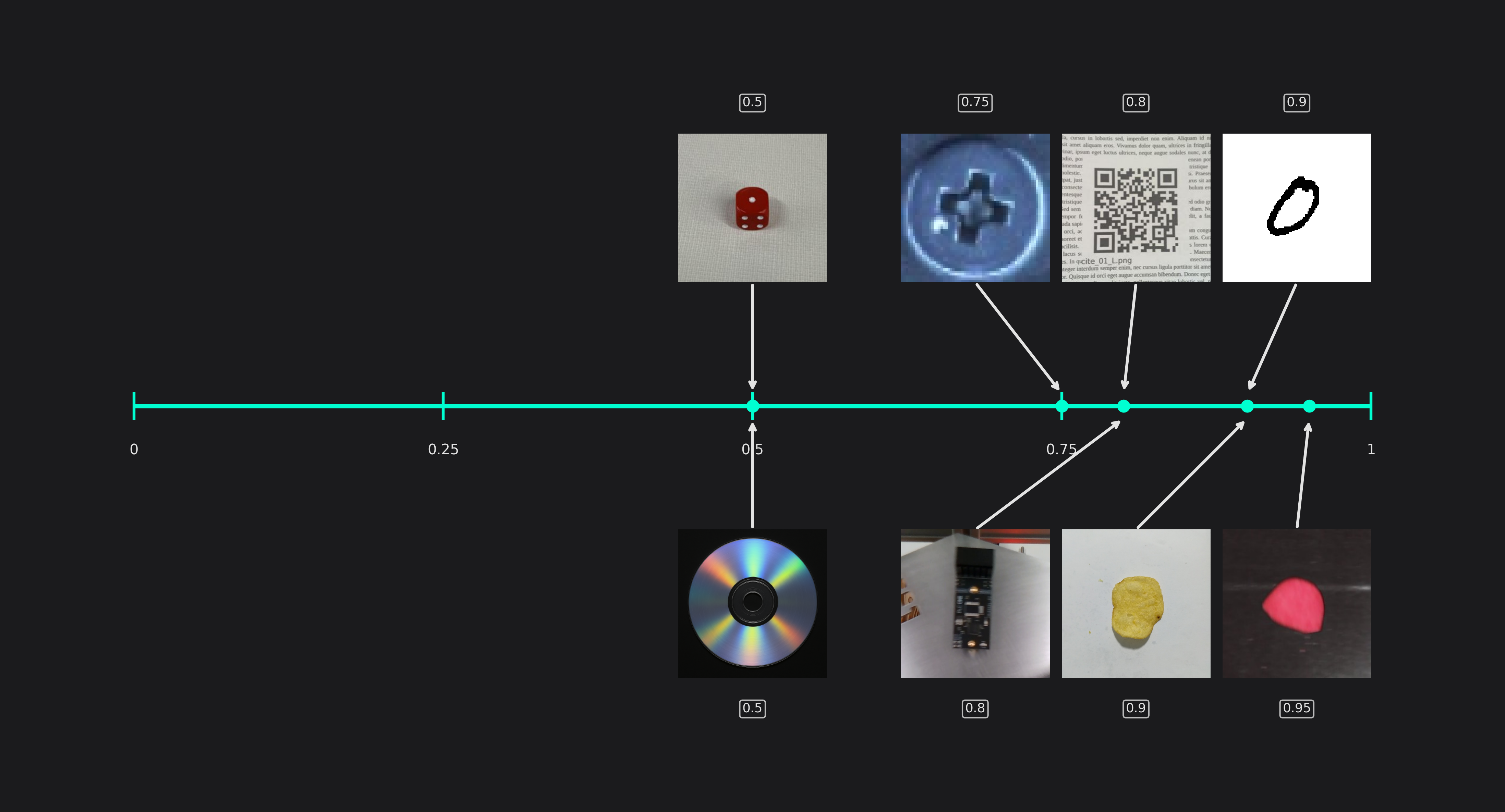
Same Class Difference
This setting describes the variance of objects from the same class. For example, two different QR-codes look quite similar while the burn marks on potato chips can be a lot more varied.

Background Difference
The background difference describes how much the image background can vary. If you take images of objects on a conveyor belt, the background will look a lot more similar than if you try to detect vehicles in traffic.

Detect Simplicity
You can use the detect simplicity to give an estimate for your task's difficulty. A high detect simplicity corresponds to simple tasks while a low value indicates a hard task.

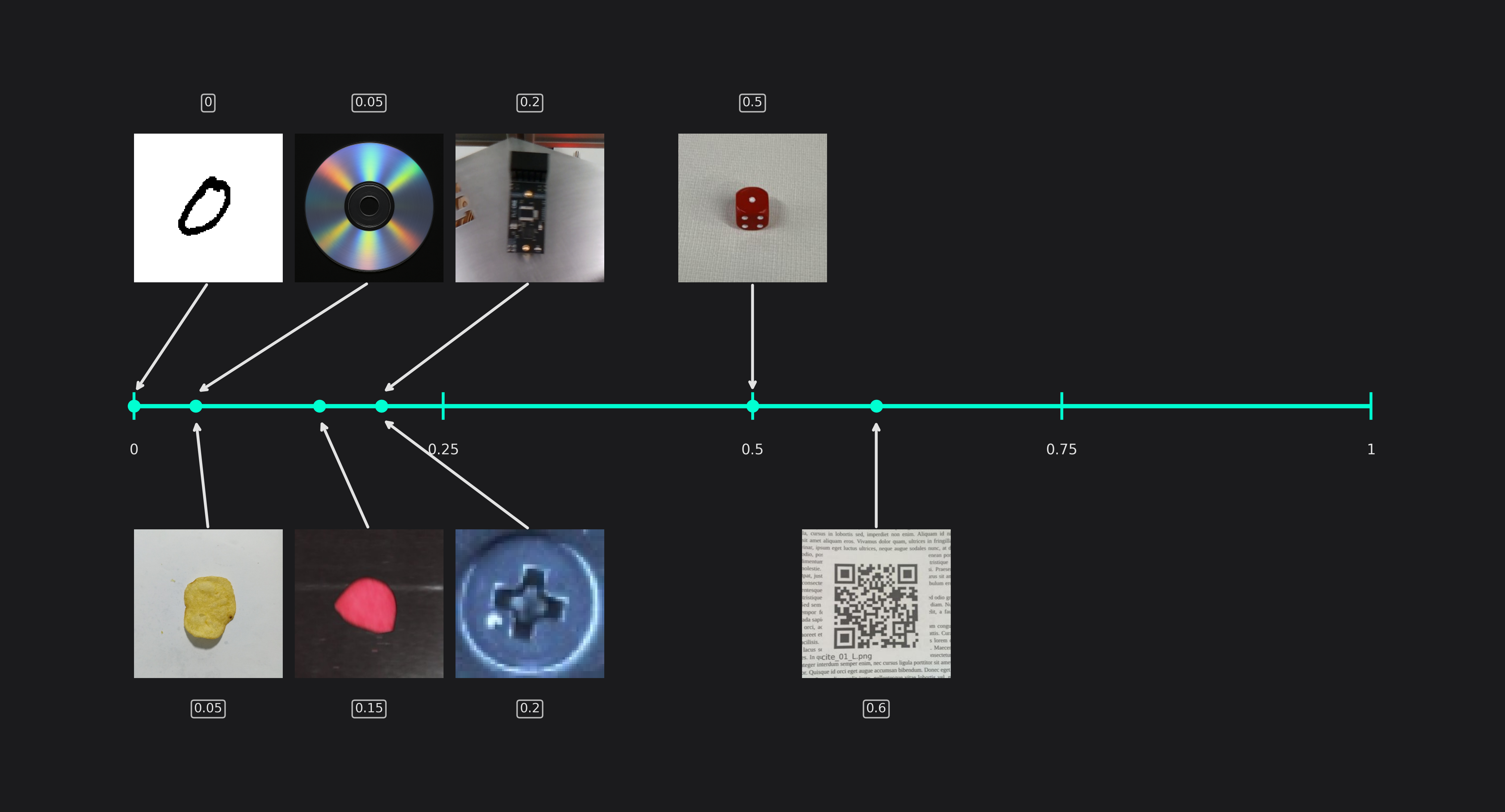
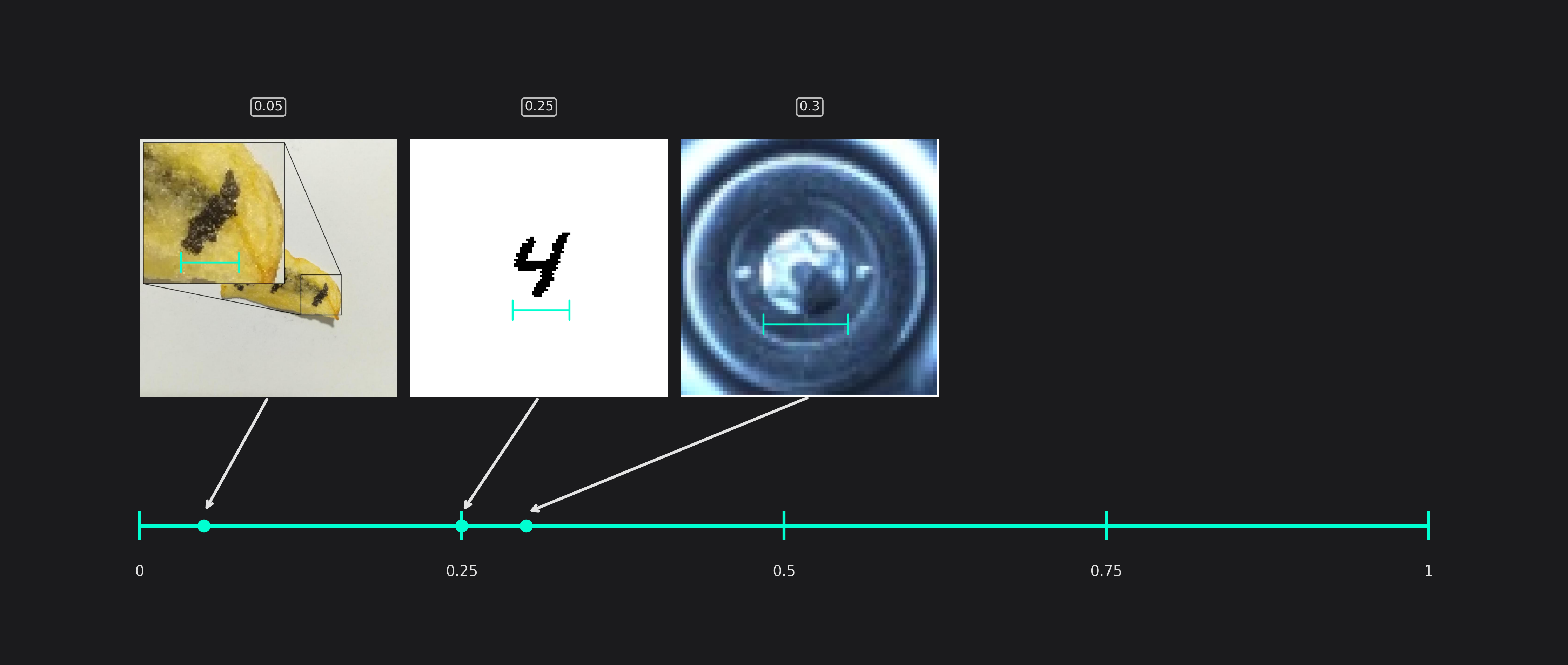
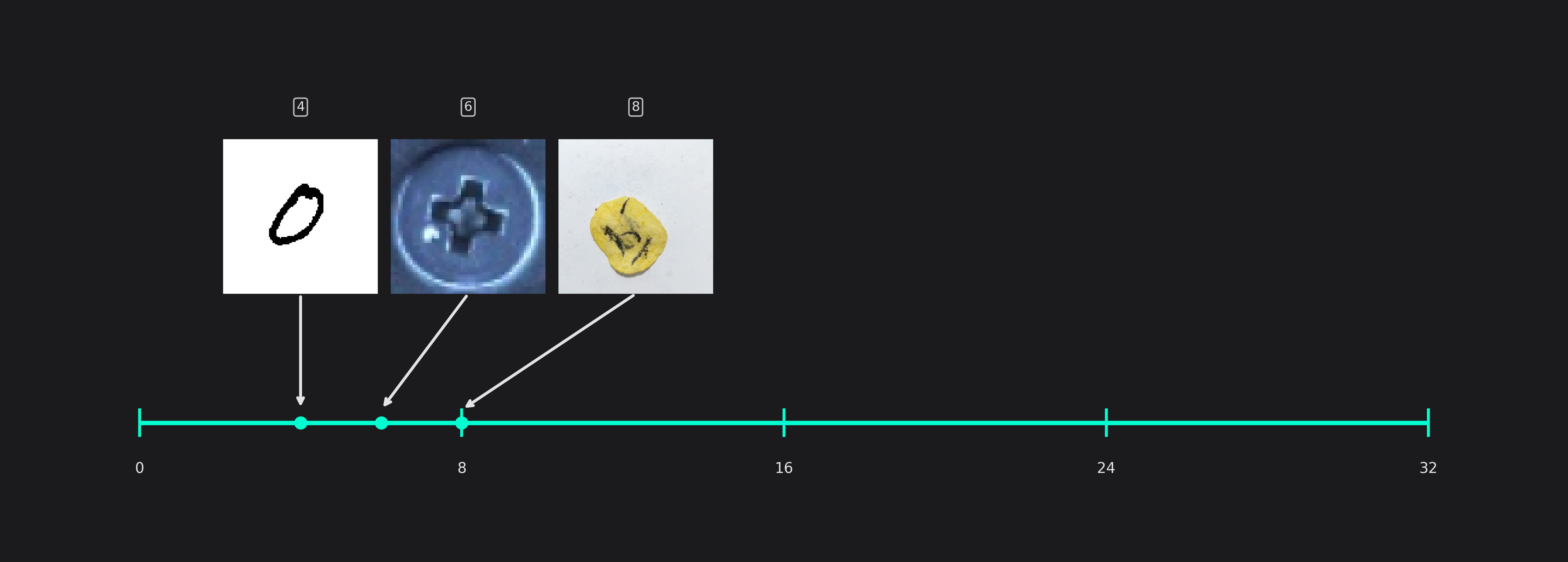
Estimated Min Object Width and Height (only used in classification tasks)
This setting specifies the size of the smallest areas that are relevant for classification tasks.

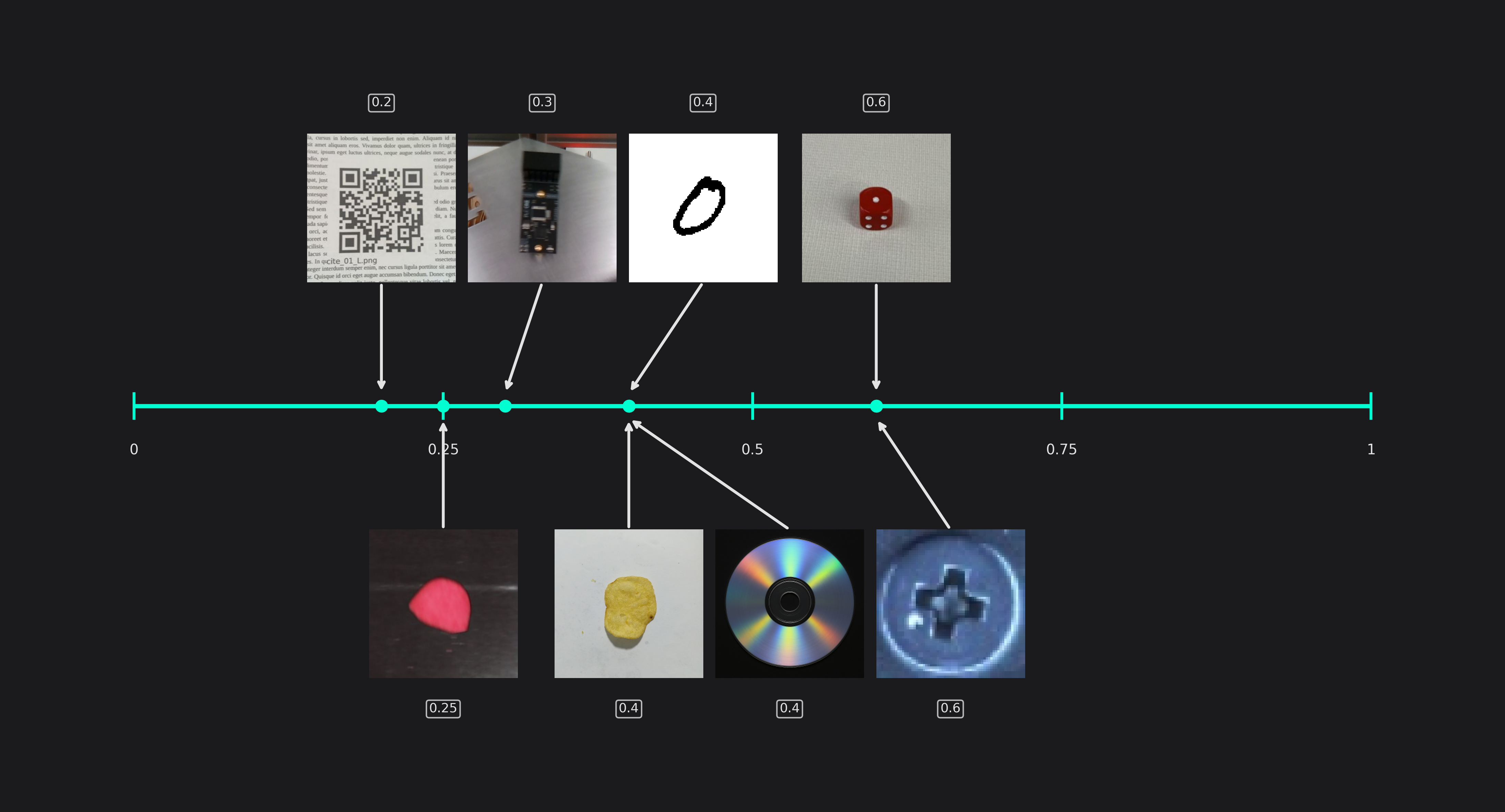
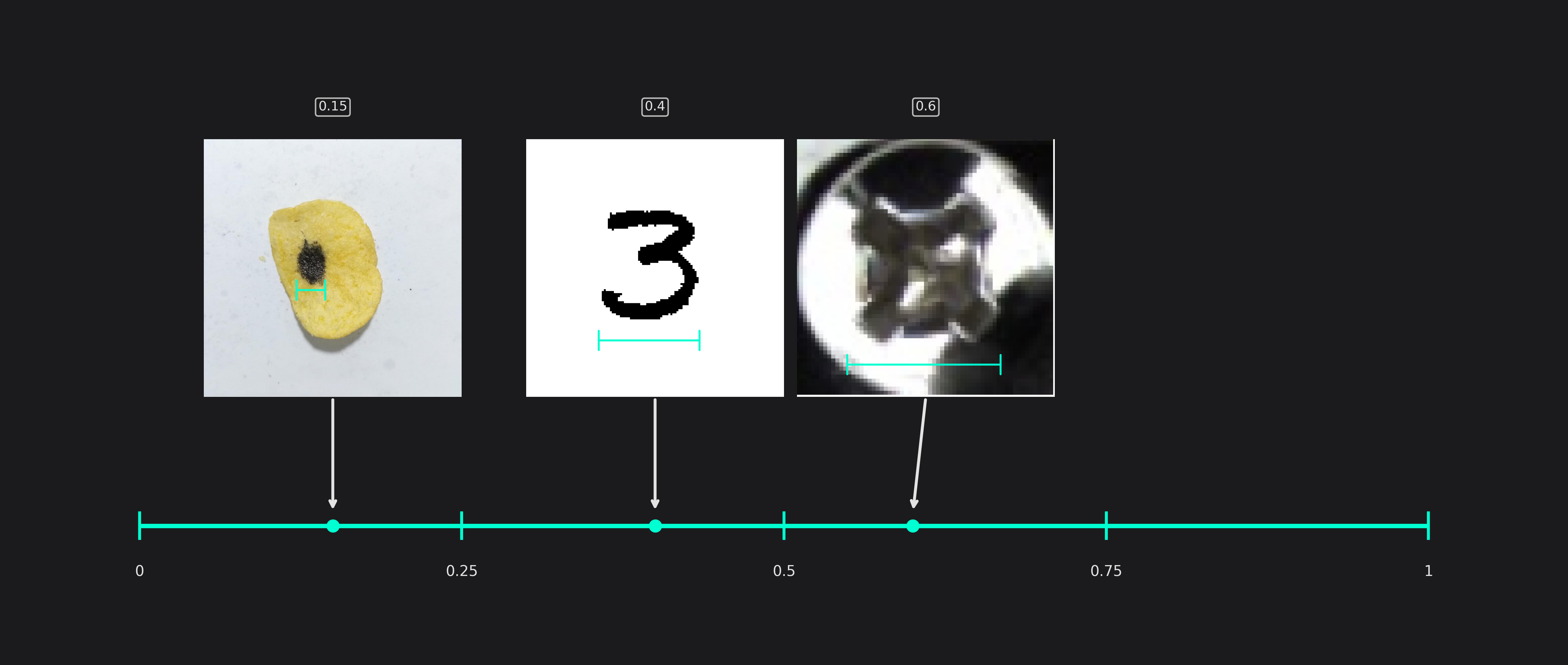
Estimated Average Object Width and Height (only used in classification tasks)
The average size of the areas that are relevant for classification tasks.

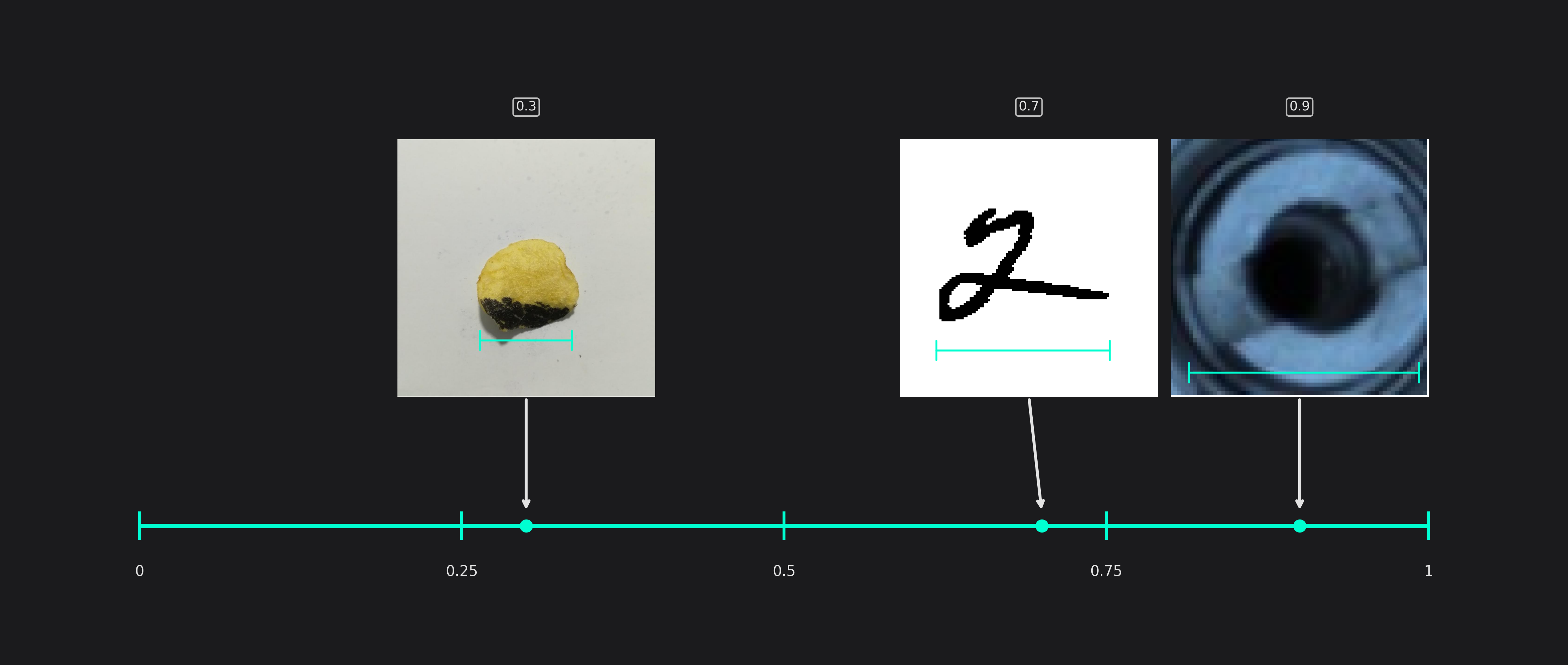
Estimated Max Object Width and Height (only used in classification tasks)
This setting reflects the size of the largest areas that are relevant for classification tasks.

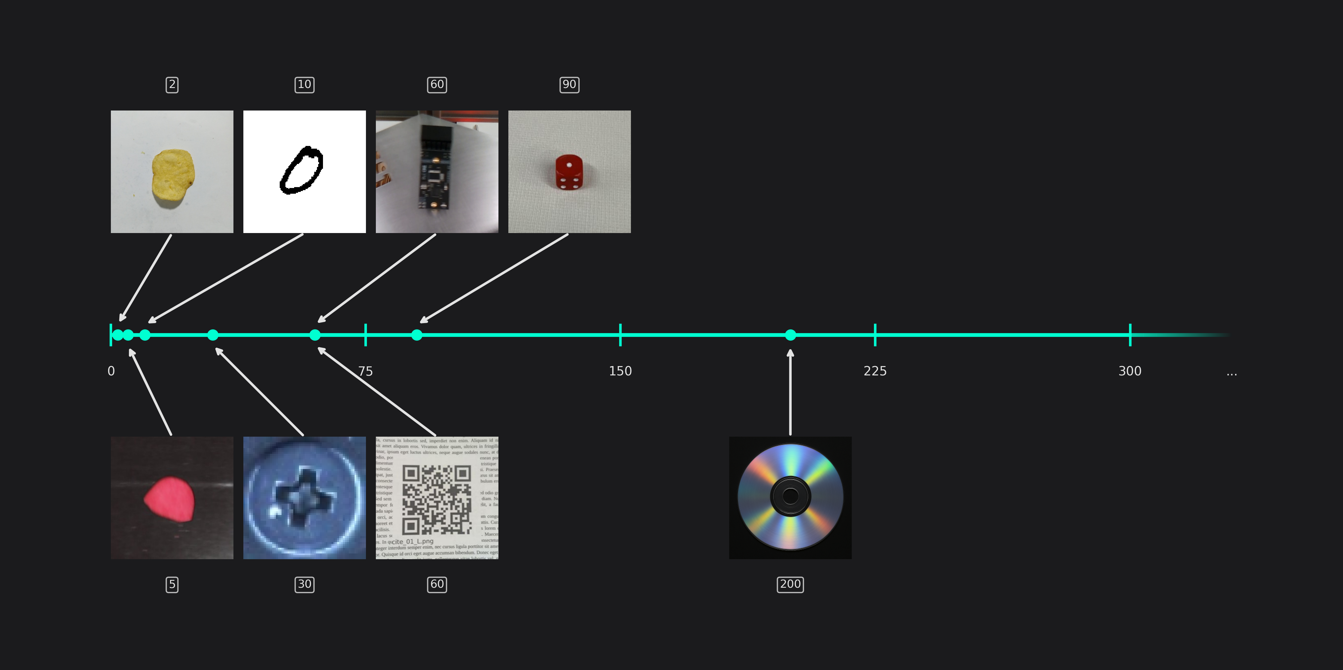
Maximum Number of Features for Classification (only used in classification tasks)
This setting describes the maximum number of image features that may be relevant for a classification task. For example, while most chips from the potato chip dataset have only a single burned area, some of them have multiple smaller burn marks. We set the value to 8 to be on the safe side.
If your task doesn't have a clear indicator, like the number of burned areas, you can use the following value ranges for orientation:

• 2-5: Simple objects with minimal variability (e.g. uniform shapes)
• 5-15: Moderate complexity with varied patterns or textures
• 20-32: Highly complex objects requiring detailed analysis

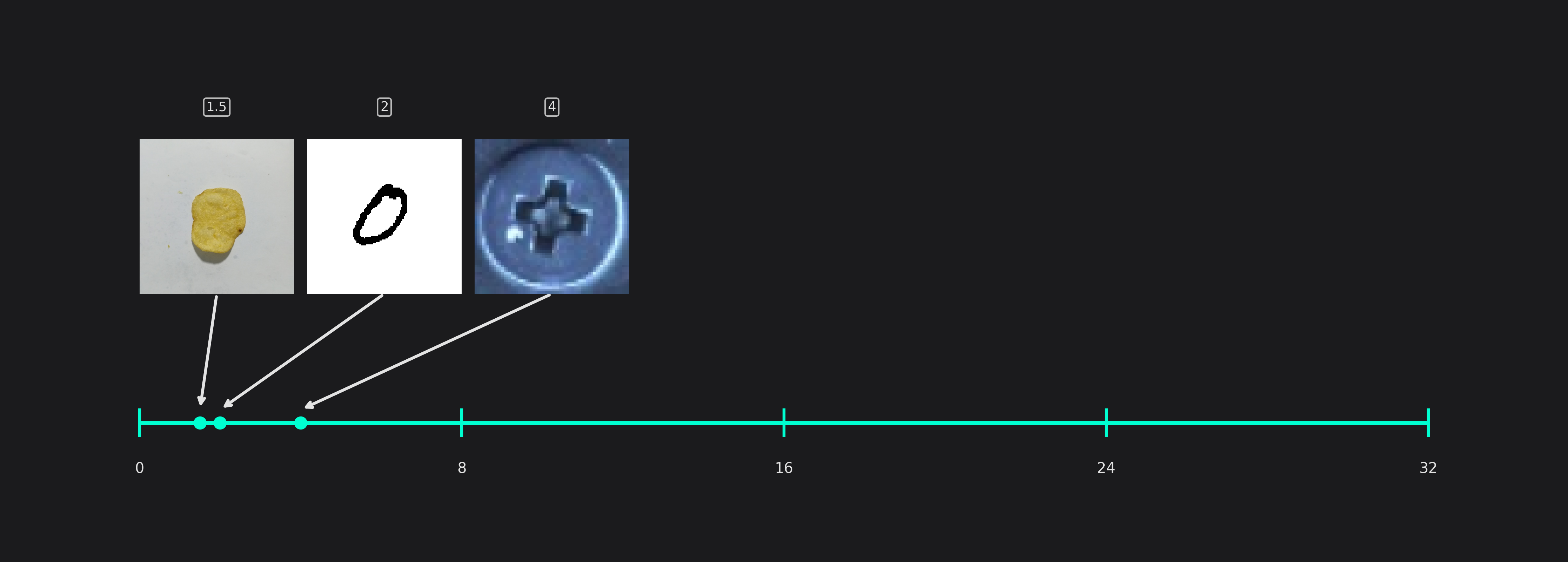
Average Number of Features for Classification (only used in classification tasks)
Similar to the last setting, this option describes the average number of features that are relevant for a classification task. For the chips example, we observed that the chips have roughly 1.5 burn marks on average.
You can use the following ranges for orientation, when you choose the value for this parameter:

• 2-4: Uniform or simple objects, e.g. identical labels
• 5-10: Moderate complexity, e.g. objects with simple textures
• 15-25: High complexity, e.g. objects with intricate details or patterns

Training

Max Training Time
This setting allows you to specify the amount of time you want to train your model. The required time depends on the complexity of the task, the size of your images, the size of the model, the amount of training data and the task itself - object detection tasks usually need more training time than similar classification tasks. The training time can range from a couple of minutes to multiple hours.

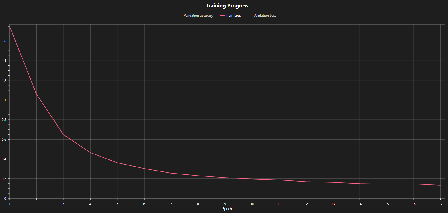
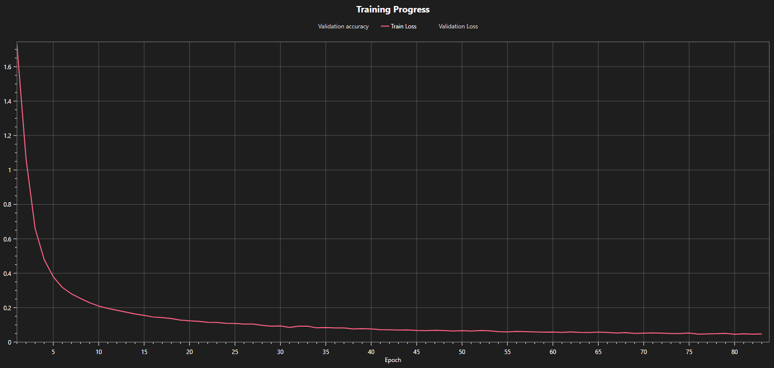
You can look at the plots of your model's training loss to see whether the training converged or needs additional time. For example, in the first graph below, you can see that the loss curve is still decreasing at the end of the training after 17 epochs. This indicates that the model is still improving and that further training will produce better results. This is confirmed in the next graph that shows the training loss for the same model but with a longer training time. The loss decreased from 0.14 at epoch 17 to under 0.05 at the end of the training. We can also observe that the loss curve is almost flat at the end, which means that further training won't yield any meaningful improvements.

Patience for Early Stopping
You can set a patience value to stop your training early if the model doesn't improve any further. The value of this setting specifies the amount of minutes over which the model shows no improvement until the training is terminated.

Percentage Quantization Optimization
If you want to export your model as a quantized model to reduce its resource requirements, you should enable quantization optimization. The corresponding slider allows you to specify the percentage of training that uses quantization aware optimization. This will improve the accuracy of the quantized model but it also reduces the training speed. If you want to achieve a good tradeoff between the required training time and model performance, we recommend setting this option to 30%. If you want to get the model with the best accuracy, you should set the slider to 100%.