Potato Chip Classification Demo

About this Demo

This demo showcases the usage of OneWare Studio and the OneAI Extension for a demo case. If you are unfamiliar with the OneAI Extension, we recommend to first take a look at our guide Getting Started with One AI.

Dataset Overview

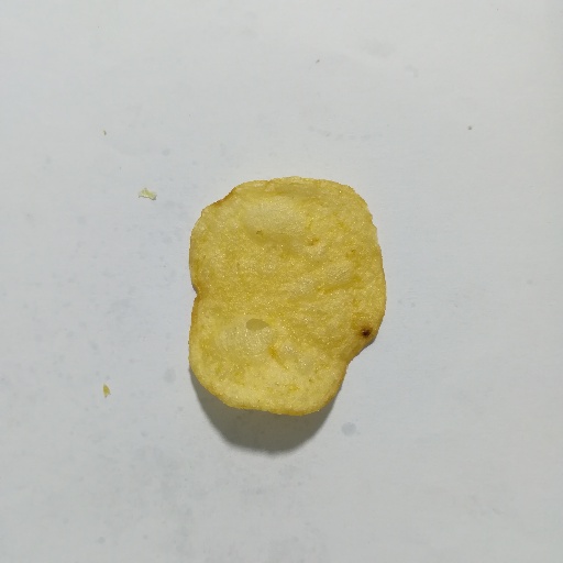
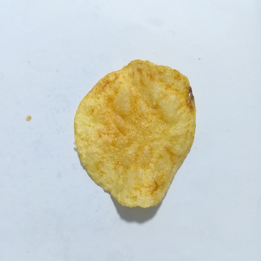
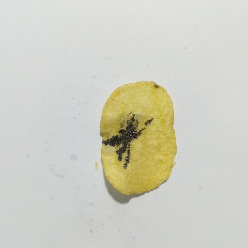
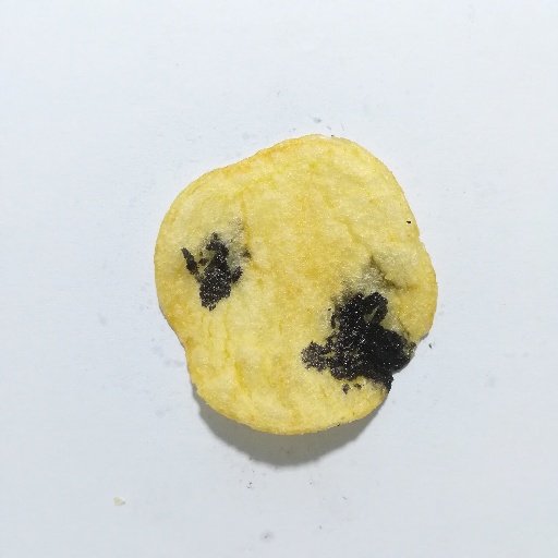
The dataset PepsiCo Lab Potato Chips Quality Control was published by the user Usama Navid on the platform kaggle. It contains quality control images from a food processing plant that produces potato chips. During the production process, the chips can get burned making them unsuitable for consumption. Our goal for this demo is to create an AI that can classify an image of a potato chip as defective or non-defective. Such an AI could be used for quality control to sort out defective chips.

Here are a few examples from the dataset:

We created a modified version of this dataset with scaled down images. This greatly reduces the size of the dataset while still keeping more than enough details to accurately classify the images. We also corrected a mismatch in the label names that would have caused an issue during the training. You can download the dataset here.

Setting up the Project and Loading the Data

First we need to create a new project by clicking on File > New > Project. To create a new AI Generator, click on AI > Open AI Generator, enter a name and select Image Detection. This automatically opens a .oneai file, which contains the settings for the AI Generator.

To load the dataset, you first need to unzip the provided dataset. Then, you need to go to the Dataset tab and click on the Import button in the top-right corner. There, you select Import Existing Dataset. In the Import Dataset window, you need to select the unzipped dataset directory, which contains the folders Test and Train. The Format of the dataset is Classification, which means that each class has its own folder containing the images that belong to that class. Since the dataset contains the folders Train and Test, the images are automatically divided into the existing train and test subsets.

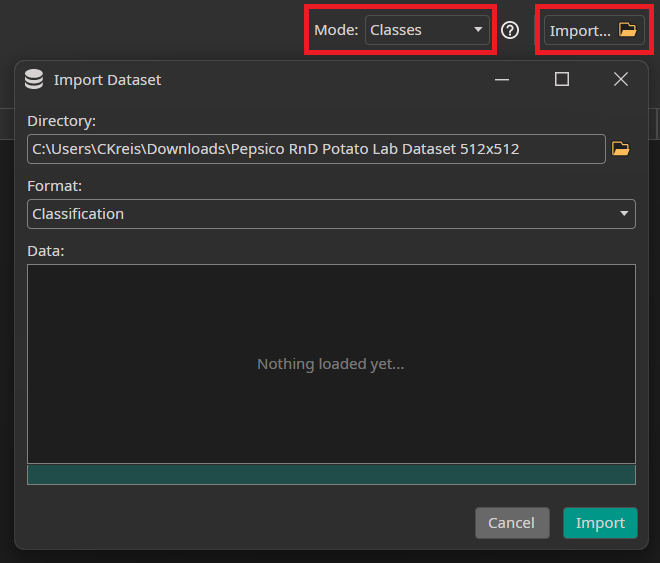
Since we want to train a classification model, we need to change the Mode from Objects to Classes. Because we don't have a predefined validation split, we let ONE AI create a validation split from the training data. The required settings are in the Validation tab but are already activated by default.

If we look into the Test tab, we see that we can reuse part of our training or validation set to increase our test set in the final model evaluation. This is useful if no or only a small test set is available, but has the disadvantage of bleeding information from the training data into the test data and thus distorting the results of the evaluation. Since the validation set is currently only used for stopping the training early if there are no further improvements, the effects should be minimal when only the validation set is reused. Reusing parts of the training set, however, will be more impactful and should only be done with caution. Because our dataset already has a separate test set, we don't need to reuse training or validation data, so we set both Train Image Percentage and Validation Image Percentage to 0%.

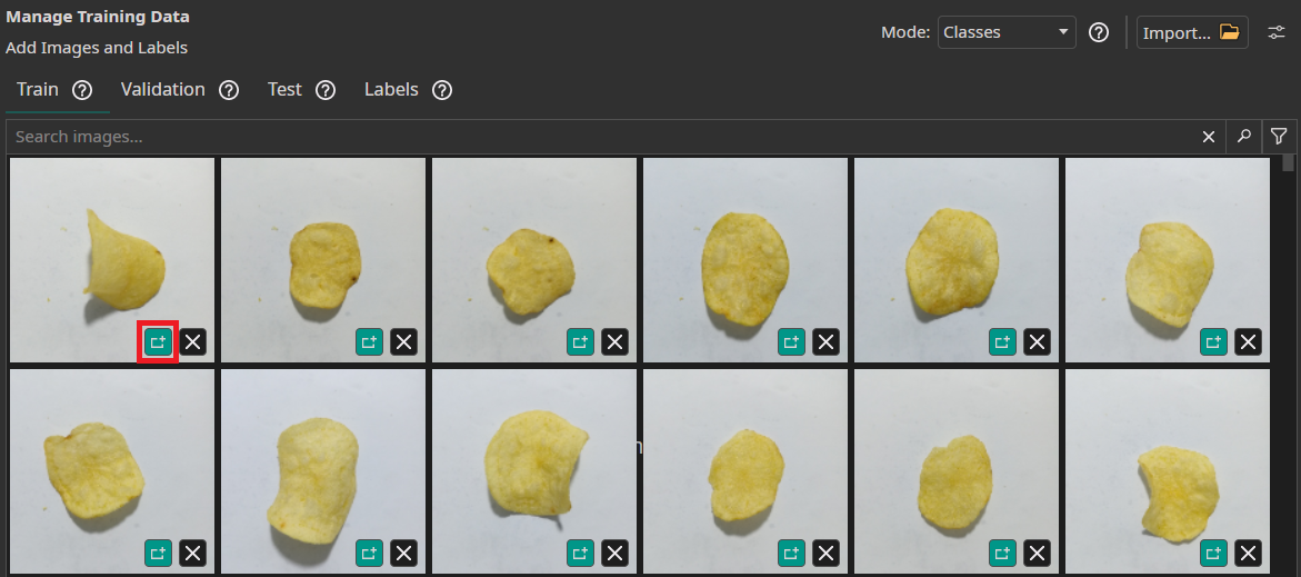
If you followed all the steps correctly, the images will show up in the Train and Test tabs of the Dataset section. Make sure that the icon for opening the annotation tool in the bottom-right corner of the images has a teal color, which shows that they are annotated.

Filters and Augmentations

Now, we need to set up our data processing pipeline by specifying the filters and augmentations. Filters are applied once to every image and are the same every time. They are used to preprocess the images. Augmentations on the other hand contain random elements and are different for every image and epoch of the training. They are used to increase the size of the dataset without the need to record and annotate new data. Furthermore, augmentations can increase the model's robustness against variations in the data by intentionally reproducing these variations. OneWare Studio allows us to set up two sets of filters - one that is applied before the augmentations and one that is applied afterwards.

For this demo, we can leave the Initial Resize filter at the default settings, because all images in the dataset have the same size. We set the Resolution Filter to 10% to reduce the 512x512 images to 51x51. This allows us to reduce the size of the images and thus the required computations while still being able to distinguish key details. For this project, we don't need any further filters.

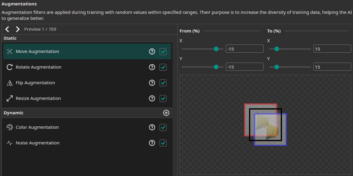
In addition, we use the following augmentations:

• Move Augmentation: This augmentation varies the images by shifting it. This makes the model more robust against shifts in the position of the potato chips. We set the amount of shift to ±15% in both directions.
• Rotate Augmentation: This augmentation rotates the images by a random amount that lies within a given range. Just like with the move augmentation, the rotate augmentation increases the model's robustness - this time against rotations instead of shifts. We set the Rotation range to ±180°.
• Flip Augmentation: The flip augmentation randomly flips the images horizontally, vertically or in both dimensions. For this demo, we select both flips.
• Resize Augmentation: The resize augmentation varies the scale of the images. We set it from 80% to 120% in both dimensions.
• Color Augmentation: The color augmentation can be used to alter the brightness, contrast, saturation, hue and gamma of the images. It helps the model to become more robust against changes in lighting. We set the Brightness adjustment to ±20, the Contrast and Saturation to (80, 120) and leave the Hue and Gamma at their default values.
• Noise Augmentation: The noise augmentation reduces the image quality by adding a noise. We reduce the settings of this augmentation to 0% and 5%.

Feel free to test around with the filter and augmentation settings. You can add additional filters and augmentations, remove them or change their parameters. Remember to set the checkmarks in the list of augmentations to enable them.

Model Settings

Now that we have set up our data processing pipeline, we configure the model settings. First, we need to specify the Classification Type. Since each image has either the class Defective or Non-Defective, we set it to One Class per Image. Next, we set the Minimum FPS to 20 and the Maximum Memory Usage as well as the Maximum Multiplier Usage to 90%. In this demo, we are going to create a model for an Altera™ Max® 10 16K, so we leave the FPGA Clock Speed at 50 MHz.

Afterwards, we provide some additional information on the characteristics of the data. First, we estimate the area the model needs to analyze to make a decision. In our example, it is enough for the model to see the burnt part of the potato chip. There is no need to analyze the whole chip. Other applications might require the model to see the whole object or even to look at the area surrounding the objects. We set the surrounding area to (10, 10) for small objects and to (30, 30) for large objects.

Next we need to estimate the difference within the same class. There is some moderate variance between the chips and their burn marks but the differences aren't huge. To reflect this, we set the Same Class Difference to 40%. The next setting describes how much the background varies. Since there is very little variation in the background, we set the Background Difference to 5%. Afterwards, we set the Detect Simplicity to 90% since the task is rather simple (easier problems have a higher value). Next, we need to tell the model the estimated sizes for small, average and large objects. We set those to (5, 5), (15, 15) and (30, 30). Finally, we need to estimate how many image features are relevant for the classification. Most defective chips contain one or two burn marks, but there are also chips with more burned areas. We thus set Average Number of Features for Classification to 1.5 and Maximum Number of Features for Classification to 8.

The last model setting is the option to organize the classes into Groups. This is an advanced setting that isn't necessary for this task, so we leave it at the default. We recommend leaving all classes in the same group unless you are certain that your task benefits from splitting the model into multiple sub-models.

Training the Model

Lastly, we set up the parameters for the hardware and the model training. In the Hardware Settings tab we select the Altera™ Max® 10 16K as the Used Hardware. If you want to deploy your model to a different kind of hardware, you can set it up here.

In the Training tab we need to click on Sync to synchronize our data and existing model trainings with the ONE WARE servers. After that, we click on Create Model to create a new model. In the next step, we select our model and click on the Train button in the top-right corner. A training time of 2 minutes is already sufficient for this task. The Patience for Early Stopping can be used to stop the training early if there are no further improvements. Since the training time for this example is so short, this setting doesn't really matter, so we leave it at the default of 100%. Since we want to export the model to an FPGA, we Enable Quantization Optimization to increase its performance. We set the Percentage Quantization Optimization to 50% so that half our training is quantization aware. The option Focus on Images with Objects is only relevant for object detection tasks, so we leave the box unchecked. The option Continue Training can be used to continue the training of a model that has already been trained. If it is unchecked, the existing model will be overwritten. Since we don't have any prior model, this setting is ignored by ONE AI.

Finally, we click on the Start Training button. You can monitor the training progress in the Logs and Statistics tabs.