Building Defects Detection Demo
About this demo
In this demo, we will build an AI model that classifies six types of building defects. You’ll learn how to tackle a complex problem using a large dataset, supported by an effective pre-filtering pipeline and targeted data augmentation to achieve results that can compete with state-of-the-art models.
Dataset overview
The BD3 Building Defects dataset was published by Praven Kottari and Pandarsamy Arjunan in the corresponding research paper, which can be found here.
It contains 3,965 RGB images covering seven annotated classes (six defect types plus a no-defect category). The authors created the dataset to support automated building inspection and address the limitations of traditional manual assessments, which are time-consuming, labor-intensive, and prone to human error. Their work presents several computer vision benchmarks that demonstrate how AI can streamline the inspection process.
In this tutorial, we will use the BD3 dataset to build an AI model following our OneAI approach, showcasing its effectiveness on a real-world problem.
To ensure comparable conditions, we use the same train, validation, and test split as in the original work, generated with the authors’ provided script, which is available in the dataset’s Github repository of the dataset.
Kottari, P., & Arjunan, P. (2024).
BD3: Building Defects Detection Dataset for Benchmarking Computer Vision Techniques for Automated Defect Identification.
In Proceedings of the 11th ACM International Conference on Systems for Energy-Efficient Buildings, Cities, and Transportation (BuildSys '24) (pp. 297–301).
Association for Computing Machinery, New York, NY, USA.
doi: 10.1145/3671127.3698789
Preparing the dataset
If you want to apply the settings of the project yourself, you need to create a new AI Generator. Click on AI > Open AI Generator, enter a name, and select Image Detection. This automatically opens a .oneai file, which contains the settings for the AI Generator.
Since the dataset is organized into class folders, we can import it as a labeled dataset. Click on Import Labeled Dataset and select the directory containing the dataset. Choose Classification as the format so the labels are automatically detected and mapped to the images. Then click Import to load the dataset.
![]()
After importing, you should see the corresponding sets under the Train, Validation, and Test tabs, as well as the seven classes listed under Labels.
Because we are using a pre-separated dataset, uncheck the Use Validation Split option and set the Validation Image Percentage at the Test section to 0%. This prevents any image from appearing in both training and testing, which would otherwise bias the results.
Filters and Augmentations
The images are already provided at a resolution of 512 * 512, which is relatively small, so we keep this size. The goal of prefiltering is to reduce the image information to what is essential —highlighting important features without removing or damaging others. For this dataset, we use a conservative prefiltering approach that slightly enhances contrast, color, and edges.
We start with a Normalize Filter to distribute the pixel values between the darkest and the lightest pixel. We increase the contrast and a bit of the color representation by adding a Color Filter and setting the Brightness to -20, the Contrast to 120, and the Saturation to 120. This makes most defects more visible. Some classes, such as Algae, benefit specifically from stronger color representation. Next, we apply a Sharpen Filter with the strength of 5, to reduce motion blur and emphasize edges. However, we apply sharpening after augmentation. In the augmentation step, we use a blur filter to simulate more realistic conditions. If sharpening were applied beforehand, the blur would undo its effect, so sharpening is performed only after all augmentations are completed.
Augmentations
This dataset is already quite large, but using augmentation helps further increase its diversity with realistic variations. In our case the pictures are already very diverse, and the defects can occur in very different representations; for example, a scratch can occur mirrored or rotated in the real world. Therefore we can apply a rigorous augmentation pipeline.
We use the following augmentations:
- Move Augmentation: We shift the picture by ±20% in both directions. Ensure that the defect is still detectable to get the best results.
- Rotate Augmentations: We let the images rotate from -180 to 180. For most defects, rotation does not affect the relevant features. While the orientation of writings could matter, our goal is only to detect the type of defect, not to read it. Additionally, in real-world scenarios, writings at the bottom of a wall could be photographed upside down, so full rotation helps the model generalize.
- Flip Augmentation: Similarly, we apply both Horizontal and Vertical flips to maximize variation. Even though flipping may not make much sense for writings, it is useful for other defects. By including both flips, we ensure the model sees defects in as many orientations as possible.
- Resize Augmentation: We apply scaling with a range of ±30% to simulate different distances from the defect.
- Color Augmentation: We set the Brightness and the Contrast to ±20. This reflects real-world scenarios, such as moving through different buildings with different light levels.
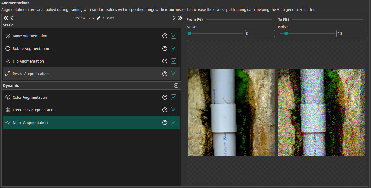
- Noise Augmentation: This augmentation makes the model robust against noise from the camera. We set the maximum value to 10%.
- Frequency Augmentation: This is also an augmentation to increase the model's robustness, in this case against blur. We let the sigma value iterate from 0% to 1%. Make sure to activate the checkbox of the low-pass filter.
Model settings
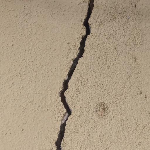
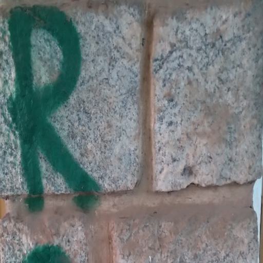
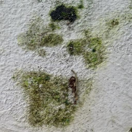
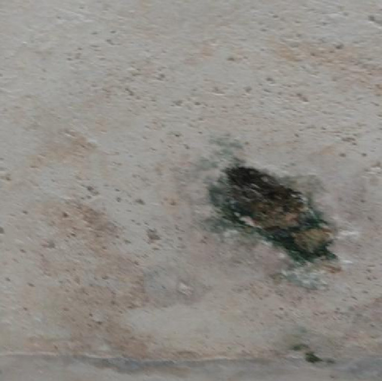
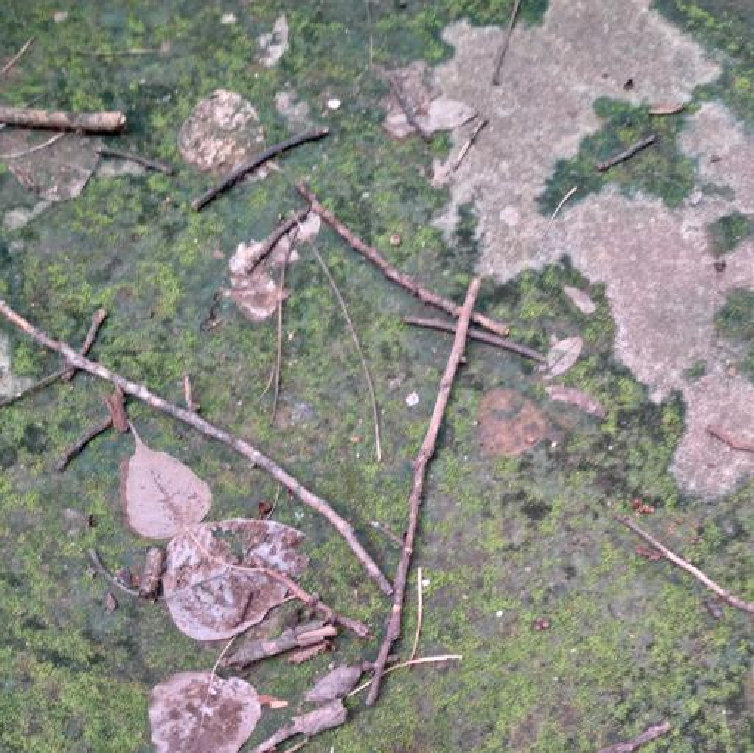
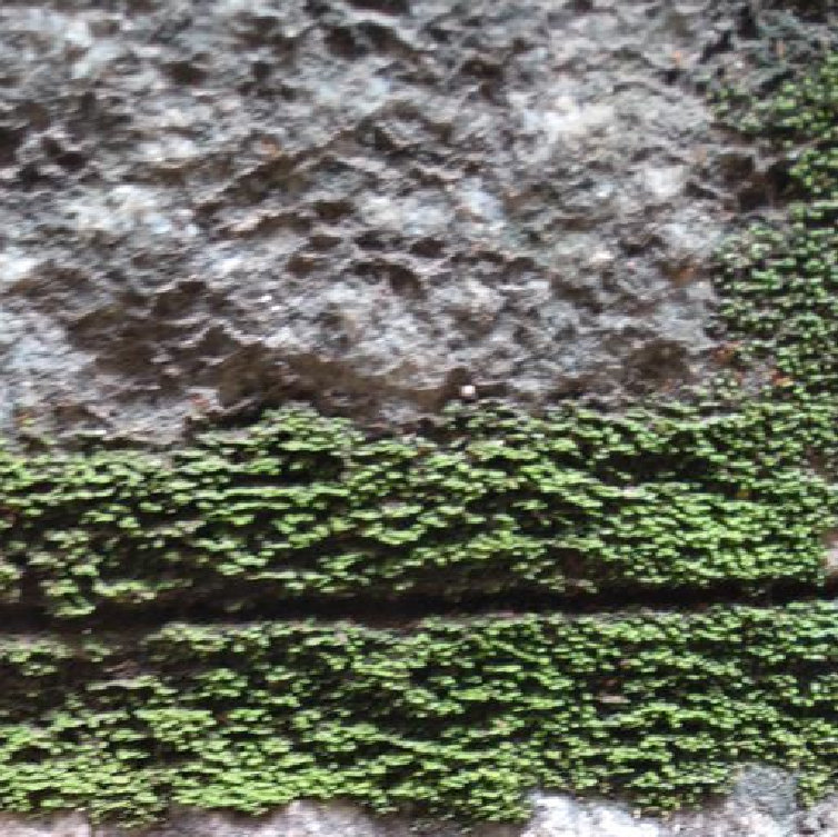
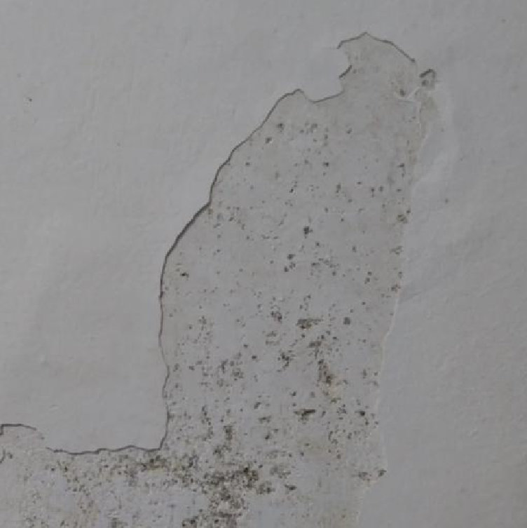
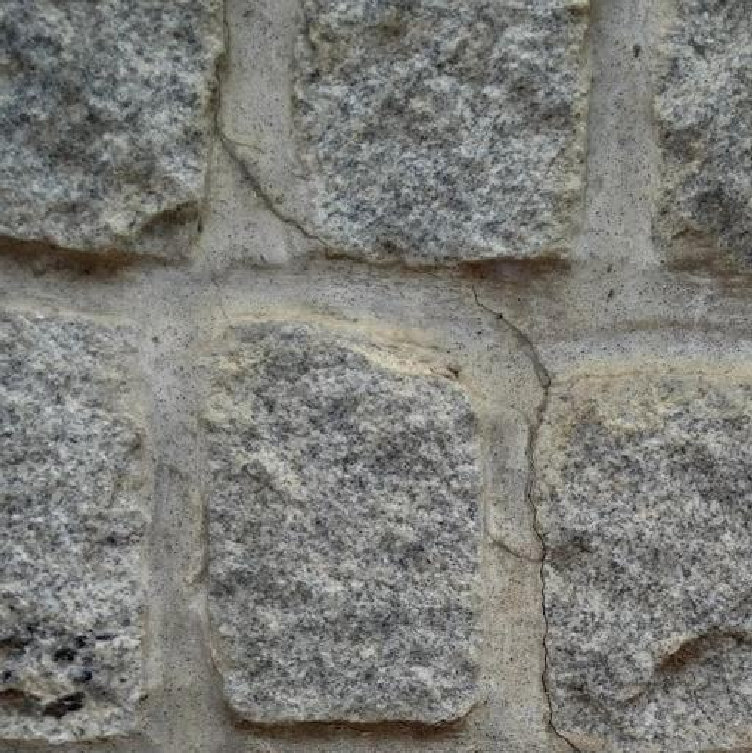
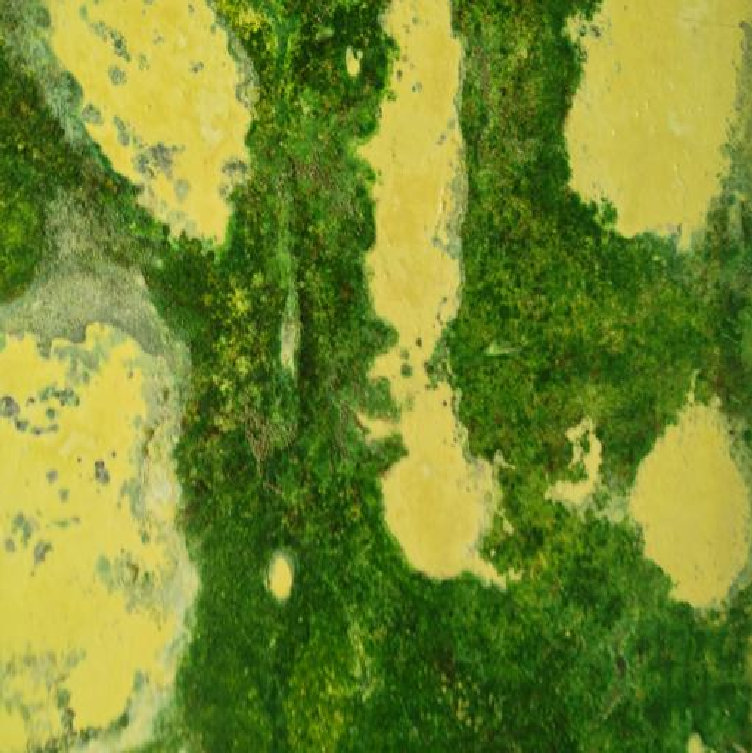
This task is challenging because the classes vary widely in size, position, and appearance of defects. Even within the same class, images can differ significantly. For example, the following three images all belong to the algae class but look very different.
To account for this, we set Same Class Difference to 80%.
We set the Background Difference to 75%, because for most pictures the background difference is very high. As shown in the pictures underneath, from left to right, the background is sometimes a plastered wall, sometimes a stone wall, and sometimes the defect fills the whole picture.
Finally, we set the Maximum Number of Features for Classification to 20 and the Average Number of Features to 12. We chose these values because the defects are not trivial and can vary significantly, for example, between the classes algae and minor cracks. To ensure the model considers a sufficient amount of relevant information, we selected comparatively high feature counts. Moreover, this is feasible because our dataset is large, which lowers the risk of overfitting, something that would otherwise increase with a more complex model architecture.
Training the model
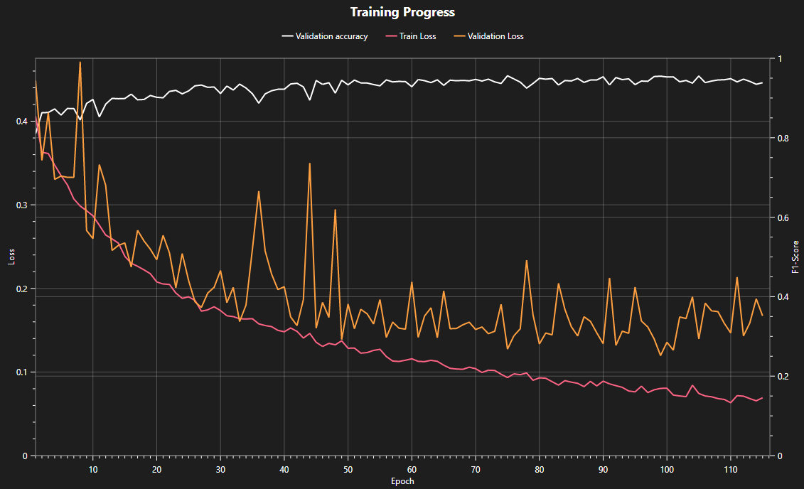
Now we can start the training process. To connect to the server, click on Sync and create a new model by clicking on the +. Click on the Train button in the top-right corner to open the training configurations. Our dataset is large and even larger with the augmentations, and our task is complex; thus, we need a lot of training time so that the model can learn from many different examples in order to detect the defects properly. We will set the training time to 30 minutes. In the logs section we can see some specifications of the model selection, e.g., the number of parameters, and under Statistics we can follow the training.
Testing the model
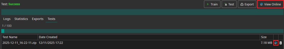
After training is complete, the model can be evaluated by clicking Test. This opens the test configuration menu, where the option Check last vs best model allows you to choose between the final trained model and the best-performing model observed during training, helping to avoid using an overfitted model.
Click Start Testing to begin the testing process. After a short time, the results will be displayed in the Logs section.
Once testing is finished, the following results were obtained for our model:
- Accuracy: 95.2%, representing the proportion of all images that were correctly classified.
- Recall: 81.4% of the images that belong to a specific class are correctly identified by the model.
- Precision: 84.5% of the images predicted as a specific class truly belong to that class.
On the one-ware cloud platform, you can also visually inspect the model's performance on the test images by navigating to Tests and clicking the internet icon or just by clicking on View Online.
Model export
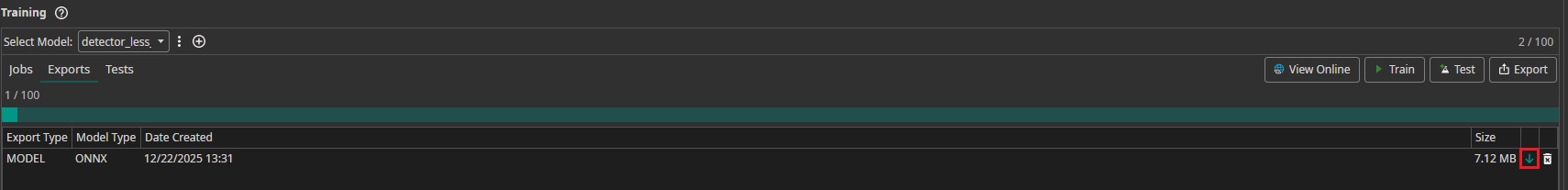
To make the model available for different tasks, you can export and download it. Click on Export to open the export configuration menu. Then, click Start Export to begin the process. Once the server has completed the export, you can download the model by clicking the downward arrow in the Exports section.
Camera tool
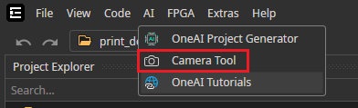
Now we want to test the performance of the model using the camera tool. With the camera tool, we can apply our trained models to live footage. You can either use a real camera or a simulated camera, which uses images from the dataset as frames. To open the camera tool, click on AI and then on Camera Tool.
For now, we will add a simulated camera. To do this, click on Add simulated camera in the top right corner and select Dataset.

This will add the simulated camera. You can adjust additional settings, such as the number of frames per second, by clicking on the gear icon.
To see the model in action, click on Live Preview. There, select the previously exported model, set the simulated camera as the Camera, choose Classification as the Preview mode, and set the Hardware to DirectML.
Now you can click on the play button to start the camera. In the bottom right corner, you can see the detected label. Next to the play button, you can see how fast the AI is running, meaning how many images the model can classify per second.

Need Help? We're Here for You!
Christopher from our development team is ready to help with any questions about ONE AI usage, troubleshooting, or optimization. Don't hesitate to reach out!