Handwritten Digit Classification Demo

About this Demo

This demo showcases the usage of OneWare Studio and the OneAI Extension for a demo case. If you are unfamiliar with the OneAI Extension, we recommend to first take a look at our guide Getting Started with One AI for Object Detection. We also recommend to read the Potato Chip Classification Demo, since it goes into more detail than this demo.

Dataset Overview

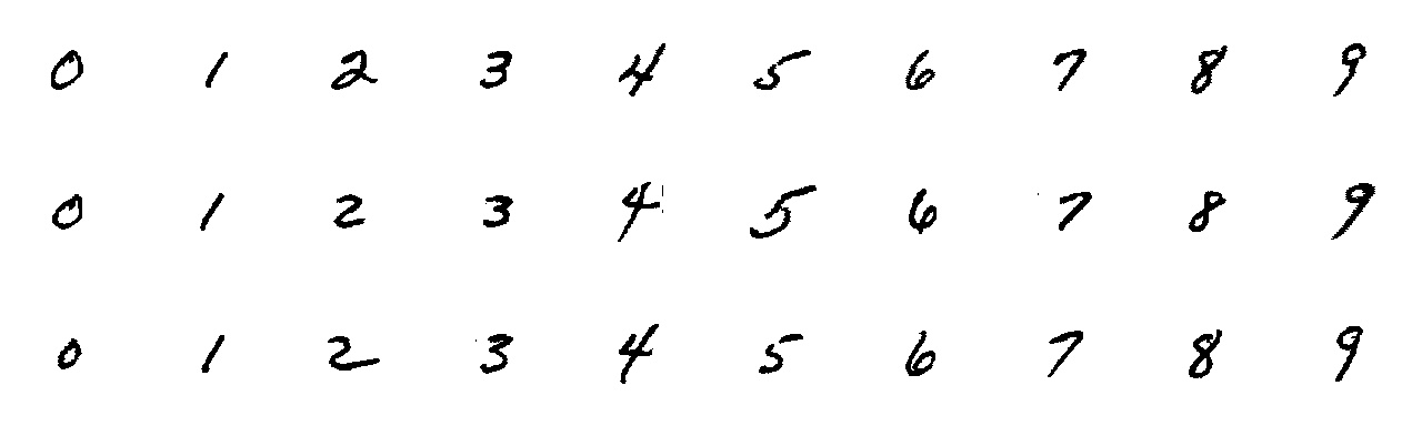
The dataset for this demo can be downloaded here. It is a subset of the NIST Special Database 19 and contains images of handwritten digits. The training set contains 3000 images, 300 for each digit, while the test set contains 500 images.

Here are a few examples from the dataset:

The goal of this demo is to create an AI model that is able to recognize handwritten digits. At the end of this demo, you will be able to test the model with live data from your webcam with your own handwritten numbers. We also provide a reference model that you can use if you don't want to train your own model.

During this demo, we will pretend that we want to train a model for an Altera™ Max® 10 16K FPGA to show the workflow and abilities of ONE AI, although the webcam demonstration will run on the CPU of your computer.

Setting up the Project

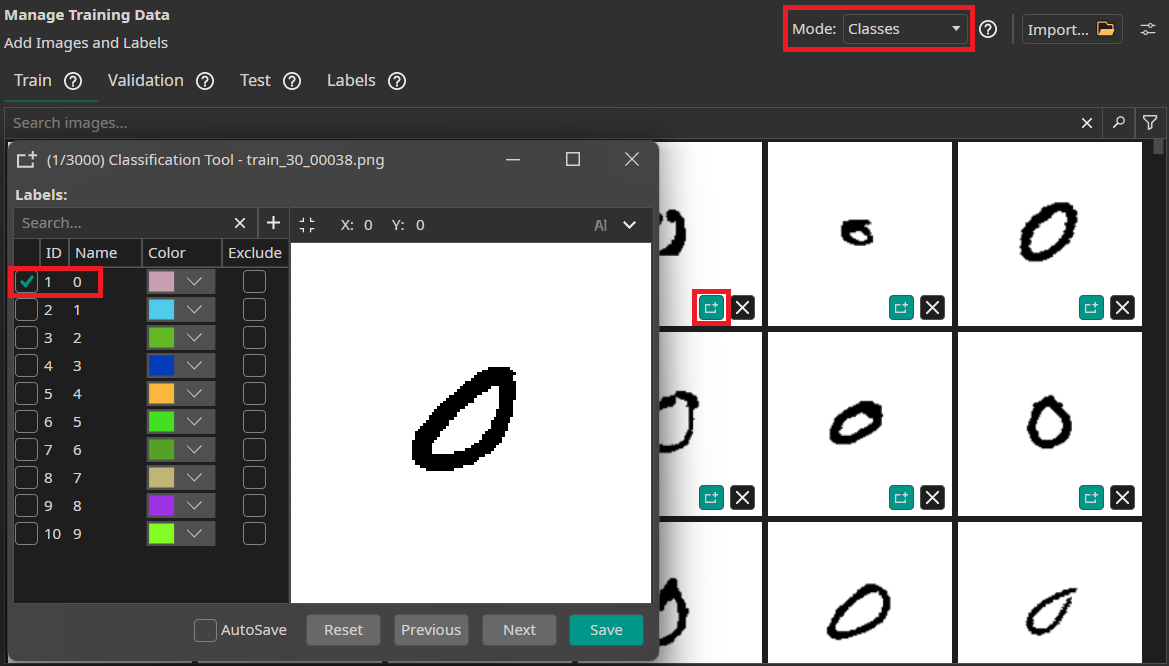
The setup process is similar to the Potato Chip Demo. First, we create a new project and a new AI Generator. Then we open the project folder in a file manager to copy the train and test data. Like before, we change the Mode to Classification and use an auto-generated validation split. Because our dataset contains a separate test set, we set both Train Image Percentage and Validation Image Percentage to 0%.

Since we want to run the model in OneWare Studio later on, we need to assign names to the labels. Otherwise, every prediction will just show "Undefined Label". To do so, we go to the Labels tab, right click the label we want to rename and click on Rename. The IDs of the annotated labels match the numbers that are visible in the images. The exception is the number zero, which has the ID 10 since the ID 0 is reserved for the background.

We can verify that everything was set up correctly by checking the annotations of our train and test images.

Filters and Augmentations

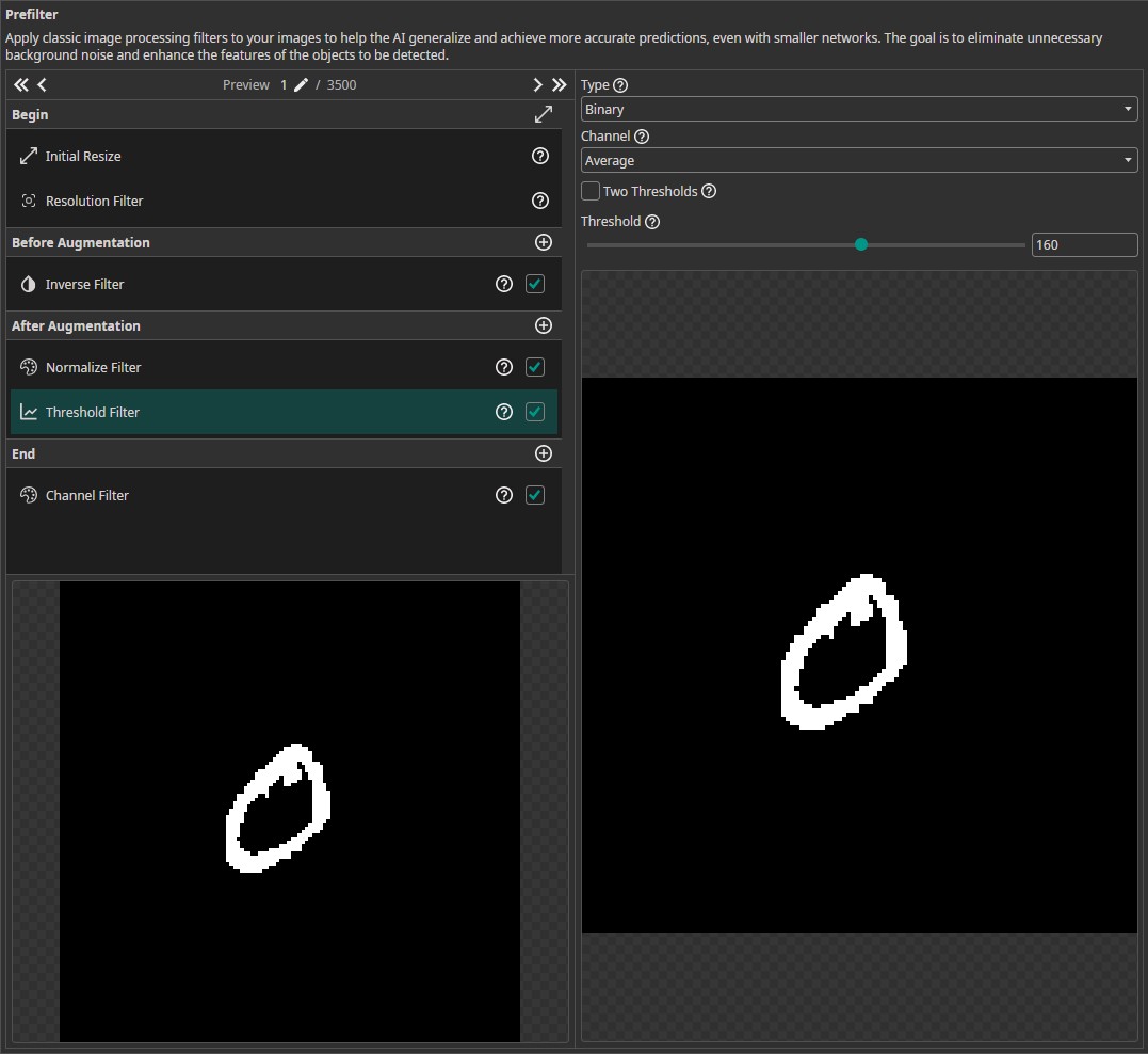
The next step is to select the filters and augmentations that we want to use. Since the size of the images is only 128x128, we don't require a Resize Filter. Instead, we apply a few other filters that will help our model with classifying the images. First, we use an Invert Filter that is applied before we augment the images. This filter converts the black numbers on a white background to white numbers on a black background. Some of the augmentations, like the Rotate Augmentation, fill missing areas with black pixels, so by using the Invert Filter, the background matches the padded areas.

In the After Augmentation section, we add a Normalize Filter. This will rescale the brightness values of the image and thus increase the robustness against lighting variations. Remember to activate the check box in the filter list as well as the box in the filter itself.

Next, we add a Threshold Filter. To achieve good results on new camera images, we increase the Threshold to 160. The other settings are left at their default values to create a Binary image based on the Average of all channels. This means that the resulting image contains only the values 0 and 255, which simplifies the classification task for our model. Additionally, this step filters out noise and lighting variations. Since the Threshold Filter reduces the images to two grayscale values, we don't need three color channels. We can remove the unnecessary channels by activating the Channel Filter in the End section and disabling any two channel.

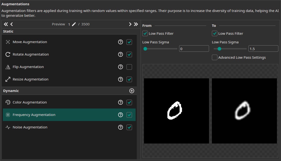
In addition to those filters, we use the following augmentations:

• Move Augmentation: We set the amount of shift to ±20% in both directions to increase the model's robustness against variations in the position of the numbers.
• Rotate Augmentation: Since numbers have a clearly defined up direction, we need a lot less rotation than in the potato chip demo. We still want to have some robustness against rotations, so we set the rotation range to ±20°.
• Flip Augmentation: We turn off the flip augmentation, since we aren't going to encounter mirrored numbers in our application.
• Resize Augmentation: Since the goal of this demo is to run the model on a webcam, our model needs to be quite robust against size variations. This is especially true for numbers that are smaller than those in the training data, because the numbers in the webcam images are likely to be smaller as well. We thus set the size augmentation from 40% to 125% in both dimensions.
• Color Augmentation: To make the model more robust against lighting variations, we add a color augmentation. We set the brightness to (-30, 30), the contrast to (80, 120) and leave the saturation, hue and gamma at their default values.
• Frequency Augmentation: We add a frequency augmentation, to simulate images that are out of focus. Thus, we only use a Low Pass Filter and set its sigma values to (0, 1.5).
• Noise Augmentation: Finally, we add a noise augmentation to increase the robustness against camera noise. This is especially useful for this dataset, because it adds some variation to the otherwise smooth background. We set the values to (0, 10).

You might wonder that some of our filters undo the effects of our augmentations. Specifically the Normalize Filter and the Threshold Filter, which will remove most if not all of the changes from the Color Augmentation as well as the Noise Augmentation. This behavior is intended. We use the augmentations to simulate variations in real life data that might not have been captured by our training data. We use filters to remove those variations that our model might encounter to increase its robustness. By using both augmentations as well as filters that counteract them, we ensure that our data pipeline is configured correctly and works in real life situations. Otherwise, we might realize during deployment that the threshold we set in the Threshold Filter removes too much or too little under different lighting conditions and ruins the model's performance.

Model Settings

After having set up the data processing pipeline, we configure the model settings. First, we need to specify the Classification Type. We want to predict one of the numbers for each image, so we set it to One Class per Image. For the tests with the webcam, it would be nice if we were able to detect multiple numbers in the same image, but since the training data doesn't contain any images with more than one number, our model won't be able to make these kind of predictions. We set the Minimum FPS to 60 and the Maximum Memory Usage as well as the Maximum Multiplier Usage to 90%. The FPGA Clock Speed is left at 50 MHz, since we are going to create a model for the Altera™ Max® 10 16K.

Next, we provide some additional information on the characteristics of the input data. First, we estimate the area that the model needs to analyze to make a decision for the smallest and the largest numbers. We set the surrounding area to (25, 25) for small objects and to (90, 90) for large objects.

Then, we estimate the variance of numbers from the same class. We observe quite a few differences in writing styles like the size, the angle or the line width, so we set the Same Class Difference to 40%. The next setting describes the variation of background. As there is no variation in the white background, we set the Background Difference to 0%. We set the Detect Simplicity to 90%, because the task isn't that complicated. Next, we need to specify the estimated sizes for small, average and large objects. We set those to (25, 25), (40, 40) and (70, 70). Finally we need to tell ONE AI how many image features are relevant for the classification. We set Average Number of Features for Classification to 2 and Maximum Number of Features for Classification to 4.

Training the Model

Now, it's time to set up the training configuration for the model. In the Hardware Settings tab we select the Altera™ Max® 10 16K as the Used Hardware.

In the Training tab we need to click on Sync to synchronize our data and existing model trainings with the ONE WARE servers. After that, we create a new training configuration. For this demo, a training time of 10 minutes is sufficient to fully train the model. We leave the patience at the default value of 30%. Since we want to export the model to an FPGA, we Enable Quantization Optimization to increase its performance. We leave the Percentage at 30% to achieve a good trade off between training time and model performance. If we want the best performing model, we need to set it to 100%, but this will increase the training time. For models that will be exported as floating point models it is best to turn off quantization.

Finally, we click on the Train button in the top-right corner to start the training. You can monitor the training progress in the Logs and Statistics tabs.

Model Export

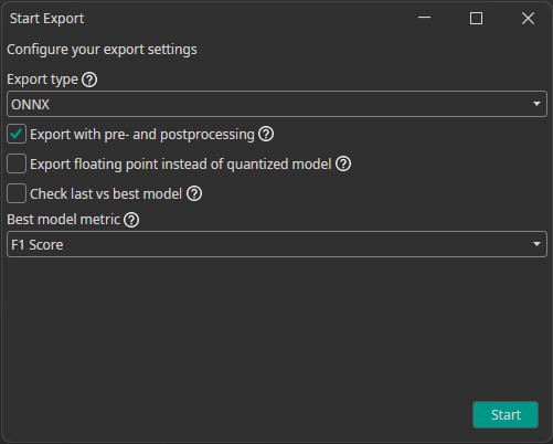
After the training is completed, we need to export our model. We configured our model to run on an Altera™ Max® 10 16K, but for now we are content with testing its capabilities on a computer. To use the model inside of OneWare Studio's camera tool, we need to export it as an ONNX model. To do so, we click on the Export button, which opens a new window with configurations. In the Export type drop-down menu, we select ONNX since that is the format we need.

Next we can activate different settings, that change how our model is exported. If we check the Export with pre- and postprocessing checkbox, ONE AI will build all of our filters directly into the model. We activate this setting, because the filter pipeline is an important part of our model. The next setting allows us to change between exporting a floating point or quantized model. At the moment, the ONNX model export supports only floating point models, so we will receive a floating point model whether we check the box or not.

The last check box allows us to select whether we want to export the last or the best model. This setting is only relevant for object detection tasks, so we can deactivate it.

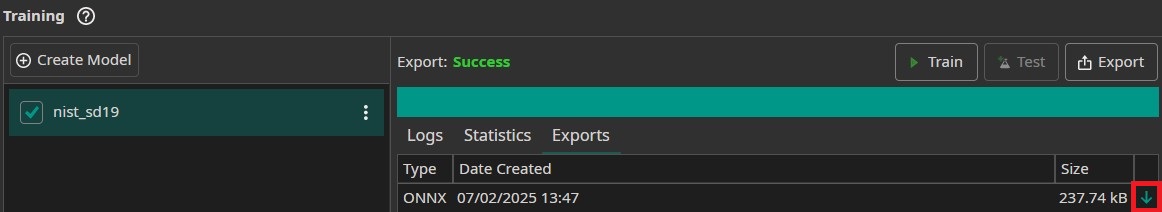
After the export is finished, we can download the exported ONNX model by clicking on the green arrow. This will save the model in the folder [selected_name]/Models. It will automatically be available to the Camera Tool that we use for testing in the next section. You can also download a trained model here. To use this model, right click on your project folder in OneWare Studio, select Open in File Manager and insert the model into the folder [selected_name]/Models. You might need to restart OneWare Studio for the model to show up in the Camera Tool.

Testing the Model

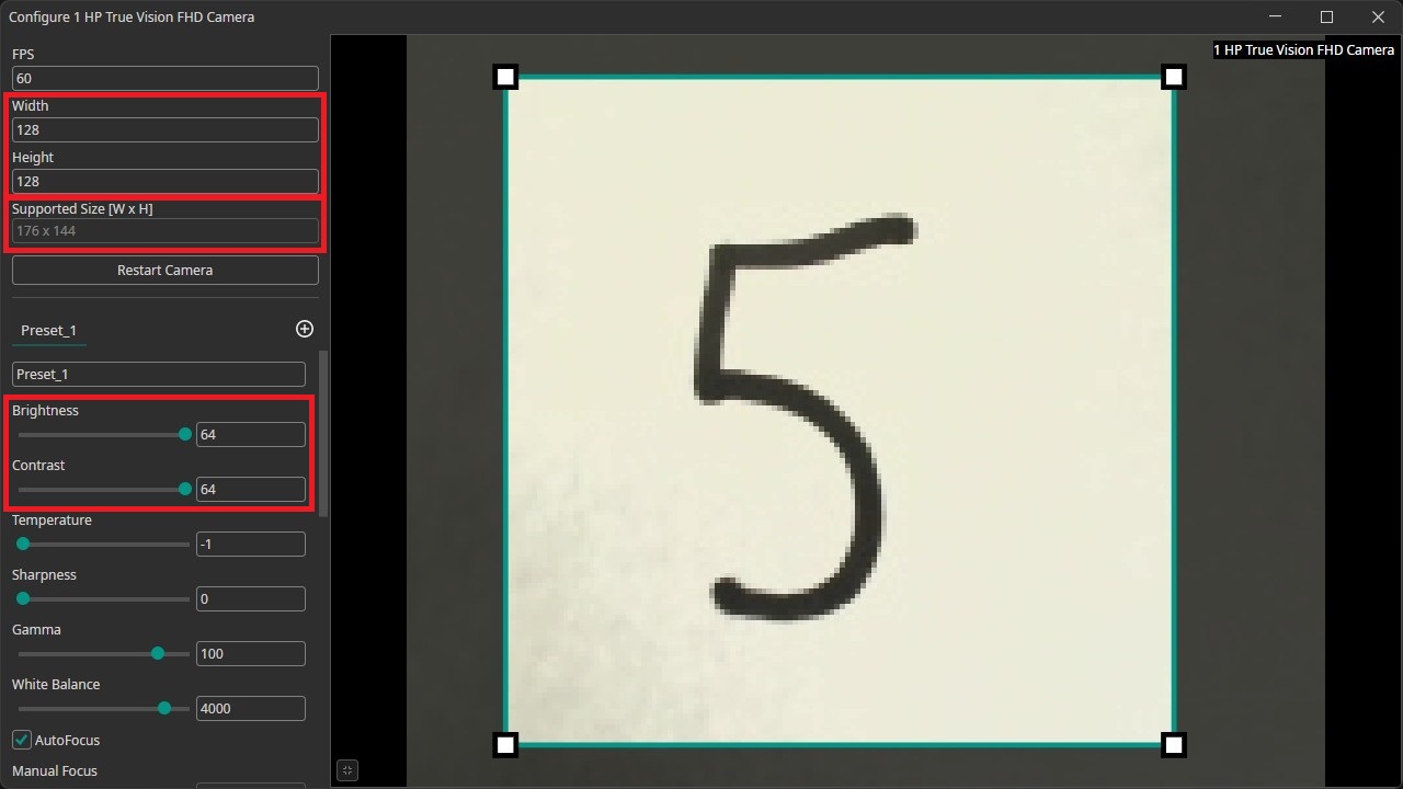
Now it's time to test our trained model. To do so, we go back to the Dataset tab and open the Camera Tool in the top-right corner. Select your camera in the drop-down menu, then click on the plus icon to add it. Next, we need to change the camera's resolution by clicking on the gear icon and setting the Width and Height to 128 to match the resolution of our images. Please check whether your camera actually supports a resolution of 128x128. You can do so by going to the Capture tab of the Camera Tool and recording an image by pressing the camera button followed by the save button. This saves the current camera image to [selected_name]/Dataset/Train. You can check its size by opening it with the Windows App Photo, which shows the size on the bottom-left. If it is larger than 128x128, you can draw a region onto the camera preview in the camera settings to crop it. It doesn't matter if the cropped region is slightly larger than 128x128, as long as it's not smaller, because that would introduce a black padding.

We can improve the classification accuracy by going to the camera settings and turning the Brightness and Contrast to their maximum. This results in the paper showing up in a bright white with a deep black number. For some cameras it is important to turn on Auto Exposure further down in the settings, because the image would be underexposed otherwise.

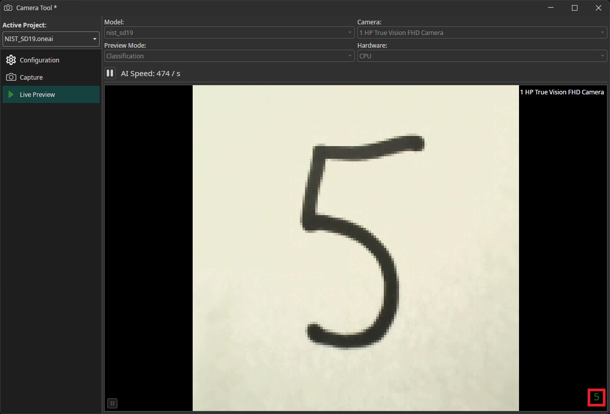
To test our model, we switch to the Run Model tab. In the drop-down menu in the top-left corner, we can select our trained model. We also need to select our camera in the top-right corner. Afterwards we click on the play-button on the top-left of the image to run the model. The predicted class will be shown on the bottom-right. You'll get the best results if you write your numbers on a white piece of paper without any markings and use a black pen with a thick line width.

Room for Improvement

You might have noticed that the model has trouble to classify some of the numbers you presented to the camera. It might be that you wrote your number in an european style, while the dataset only contains numbers that are written in an american style. There are differences for the numbers one, seven and nine. The european version of the number one consists of two lines while the american version contains only a single line and the european seven typically has a horizontal line that is missing in the american seven. The difference between the two versions of the number nine is a bit more subtle. Europeans usually add a curved hook at the bottom of the number while americans draw a straight line.

Even though these differences might seem trivial to us, the model is struggling with them. For our model, this effect is especially strong with the number nine. It is often mistaken for the numbers three or five, because those numbers have a curve at the bottom that is similar to the bottom of the european nine.

This observation shows the importance of collecting a dataset with many variations. If an important feature doesn't occur in the training data, the model won't know what to do with it, which typically results in low quality predictions. This is also the reason why we use augmentations. By introducing variation into the training data, the model becomes more robust against these types of variation.

You might recall that the dataset we provided to you is a small subset of the full NIST Special Database 19. When we selected the training images, we took the first 300 images for each digit. Because the dataset is sorted, we only selected numbers from a small subset of people resulting in small variance in our data. We created a second dataset, which contains randomly selected samples. You can download the dataset here as well as a trained model here. When you look at the images, you'll see that they feature a much higher variance in writing styles. You'll also notice that the new model is a lot better at detecting the number nine.