Dice Detection Demo
About this Demo
This demo showcases the usage of OneWare Studio and the OneAI Extension for a demo case. If you are unfamiliar with the OneAI Extension, we recommend to first take a look at our guide Getting Started with One AI. We also recommend to read the Potato Chip Classification Demo, since it goes into more detail than this demo.
Dataset Overview
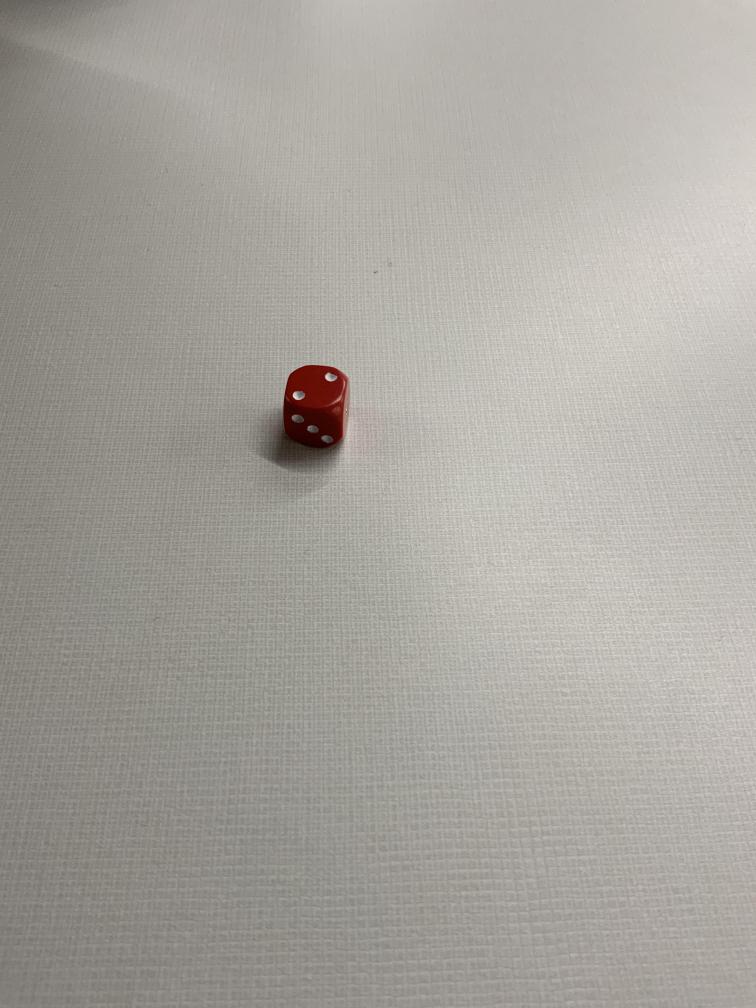
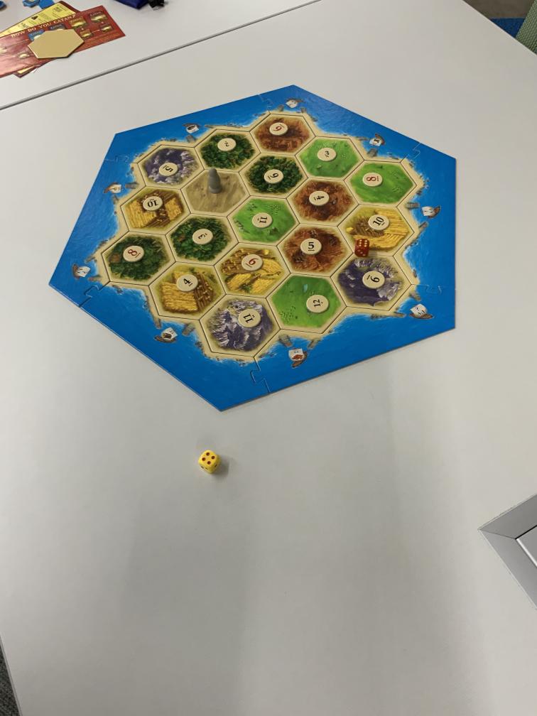
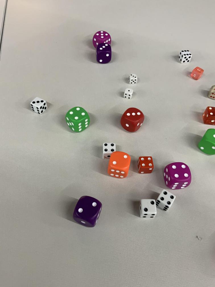
The 6 Sided Dice Dataset was published by Roboflow and contains 359 images of six-sided dice. The data set contains multiple dice of differing colors and size. 160 images contain a CATAN board underneath or near the dice - the other images feature a white table as the background. Most of the images contain only one or two dice, but there are also 13 images containing a mass grouping of dice.
Here are a few examples from the dataset:
We created a modified version of this dataset with annotation files that are compatible with the current version of the OneAI Extension. You can download the dataset here.
Setting up the Project
The setup process is similar to the Potato Chip Demo. First, we create a new project and a new AI Generator. Then we open the project folder in a file manager to copy the training data. Since this demo deals with an object detection task we leave the Mode at Annotation and do not change it to Classification like before. In the Validation tab, we set up an auto-generated validation split that we set to 30% due to the small size of the dataset. We don't have a separate test set for this dataset, so we go to the Test tab and ensure that the Validation Image Percentage is set to 100%.
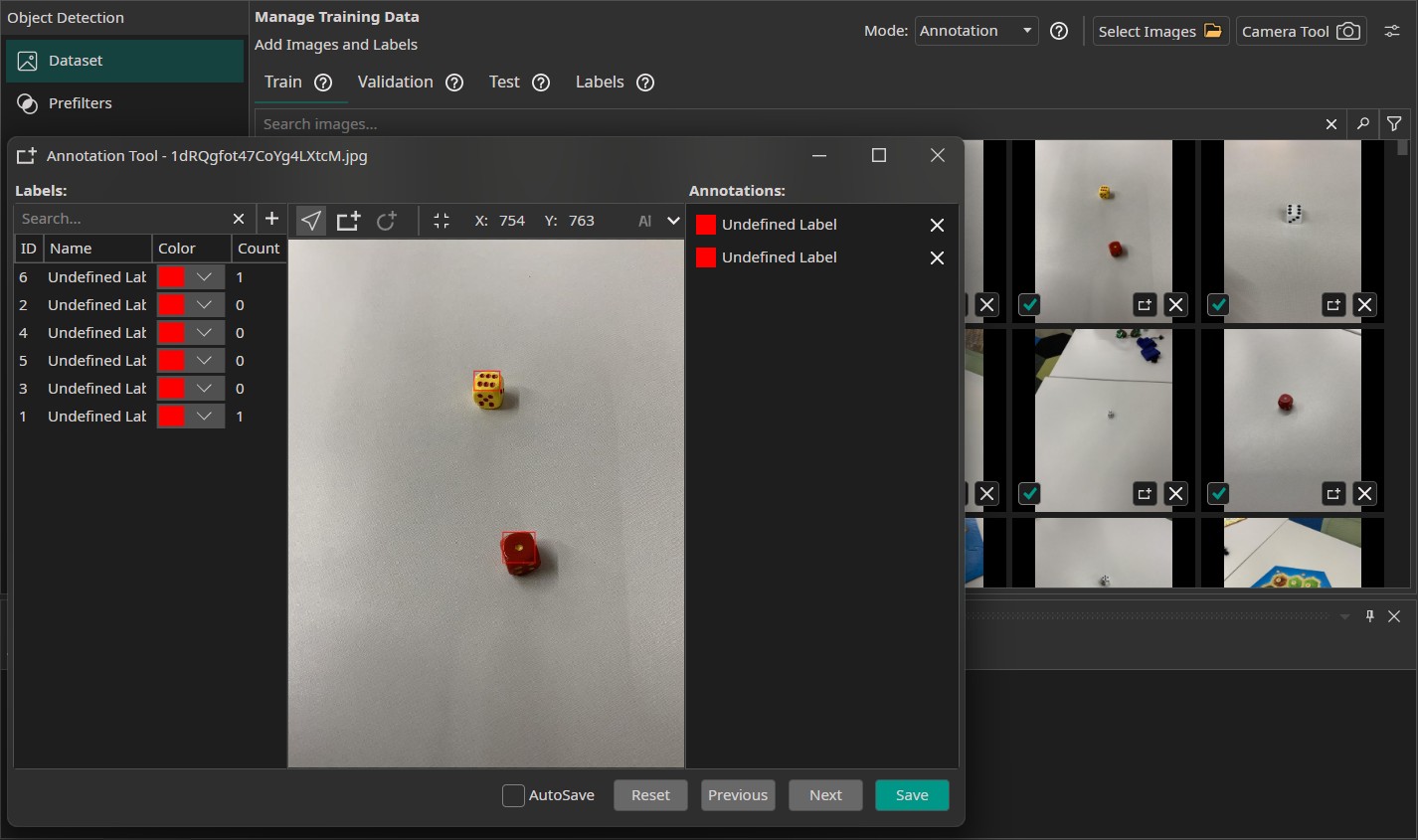
We can verify that everything was set up correctly by checking the annotations of our train images. It is expected that the labels are named "Undefined Label", since we never specified a name. We can do so in the Labels tab or when viewing a annotation but that isn't necessary.
Filters and Augmentations
Now, we select the filters and augmentations that we want to use. Since the dice are quite small in some of the images, we can't reduce the image size without sacrificing performance. Unfortunately, this means that we can't use a Resize Filter to reduce the amount of computations. The only filter that we are going to use in the demo is a Sharpen Filter, which is set to 10, to make the dots of the dice easier to see.
In addition, we use the following augmentations:
- Move Augmentation: We set the amount of shift to ±20% in both directions.
- Rotate Augmentation: We set the rotation range of the rotate augmentation to ±10° since rotational robustness doesn't have a major importance for this demo.
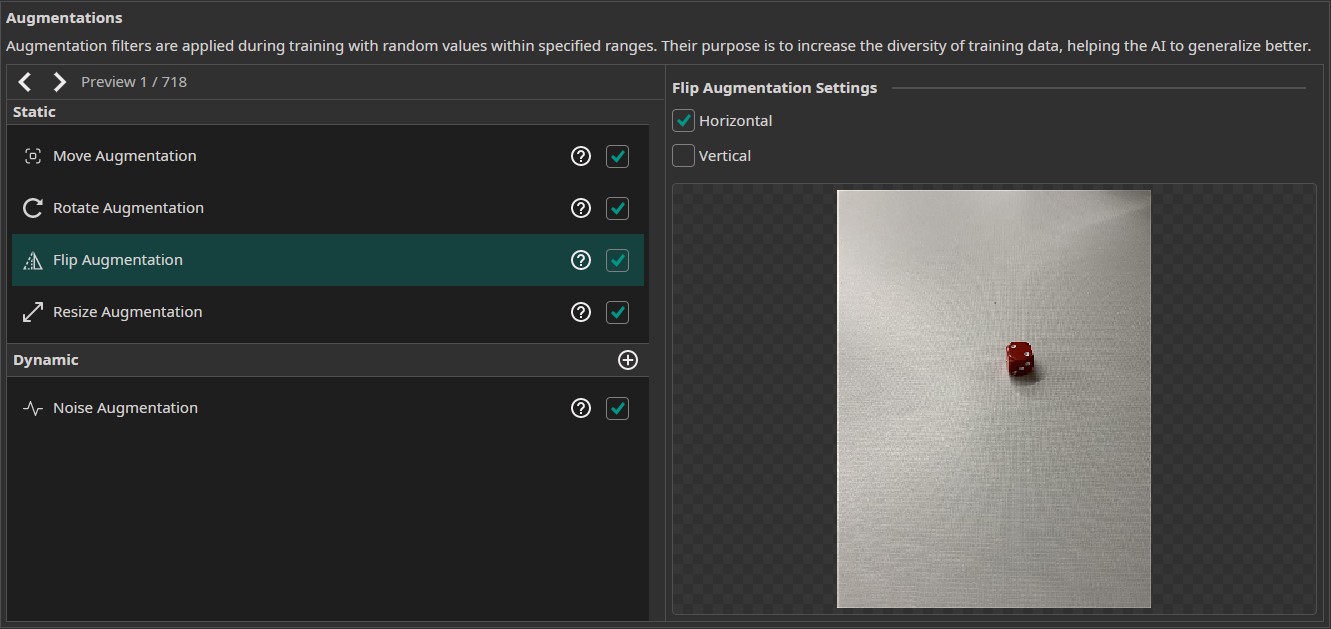
- Flip Augmentation: For this project, we only select horizontal flips. Since the dice weren't photographed straight top-down but at an angle, using vertical flips would change the perspective of the images.
- Resize Augmentation: We vary the size from 80% to 120% in both dimensions to make the model more robust against changes in the object sizes. This could happen due to the dice being different distances away from the camera or them having different sizes.
- Noise Augmentation: We add a noise augmentation and reduce the settings to 0% and 5%.
Model Settings
Our next step is to configure the model settings. Our goal is to detect bounding boxes around the dice, so we select the Prediction Type to Size, Position and Class of Objects. We prefer to have an accurate prediction but don't require it to be perfect, so we set the X/Y Precision to 50% and the Size Precision to 25%. We don't want to prioritize precision nor recall, so we select the balanced approach and leave the Prioritize Precision slider at 50%. Next, we can specify the performance requirements of the model. We set the Minimum FPS to 20 and the Maximum Memory Usage to 90%. Since the model isn't exported to an FPGA, the settings for the Maximum Multiplier Usage and the FPGA Clock Speed aren't used.
Afterwards, we provide some additional information on the characteristics of the data. We estimate that the required surrounding area for small objects is (10, 8) and (20, 16) for large objects. Since the sides of the images aren't of equal length, these settings result in areas that are roughly square.
Next we need to estimate the difference within the same class. For our example, this translates to "How different are two images of a dice that show the same number?". At the first glance those images look quite similar, but if we look more closely we notice that there are some differences. The dice have different sizes and colors - some are even slightly translucent. Furthermore, the dices are photographed from different angles. Some images show only the top face while others also show one or two side faces. The images of the mass groupings even contain dice that show numbers instead of dots. To capture this complexity we set the Same Class Difference to 75%.
Afterwards, we need to give an estimate for the background variance. While the images that have a white table as the background vary little, the images showing the CATAN board feature a lot of variance. To reflect this, we set the Background Difference to 50%. Since the dice need to be detected from different angles and distances as well as in changing situations with a varying amount of dice, this task is surprisingly complex at a closer look. It is placed somewhere between a moderate and a high complexity, so we set the Detect Simplicity to 25%.
Training the Model
Finally, we set up the parameters for the model training. In the Hardware Settings tab we set the Used Hardware to Default GPU.
In the Training tab we need to click on Sync to synchronize our data and existing model trainings with the ONE WARE servers. After that, we create a new training configuration. Object detection tasks tend to need a lot more training than classification tasks so we set the training time to 60 minutes. The patience is set to 25% to terminate the training early if there are no further improvements. Since we don't plan to export the model to an FPGA, we don't need to enable quantization.
Finally, we click on the Train button in the top-right corner to start the training. You can monitor the training progress in the Logs and Statistics tabs.